CenterNet代码原理详解
零、序言
版权声明:此份电子书整理自公众号「GiantPandaCV 」, 版权所有 GiantPandaCV , 禁止任何形式的 转载, 禁止传播、商用, 违者必究! GiantPandaCV 公众号由专注于技术的一群 90 后创建, 专注于机器学习、深度学习、计算机视觉、图 像处理等领域。半年以来已更新 242 篇原创技术文章。我们编写了 《从零开始学习YOLOv3》 、《从零开始学习SSD》 、《Faster R-CNN原理和代码讲解》 、《多目标跟踪快速入门》等系列原创电子书,关注后回复对应关键字即可免费领取。每天更新一到两篇相关推文, 希望在传播知识、分享知识的同时能够启发你。 欢迎扫描下方二维码关注我们的公众号。

一、训练自己的数据集
这书是基于非官方的CenterNet实现,https://github.com/zzzxxxttt/pytorch_simple_CenterNet_45,这个版本的实现入门难度小一些,基于官方版本(https://github.com/xingyizhou/CenterNet)进行修改,要比官方代码更适合阅读和理解,dataloader、hourglass、训练流程等原版中比较复杂的部分都进行了重写,最终要比官方的速度更快。
本章主要讲解如何用这个版本的CenterNet训练自己的VOC数据集,环境的配置。
1. 环境配置
环境要求:
- python>=3.5
- pytorch==0.4.1or 1.1.0 or 1.0.0(笔者用的1.0.0也可以)
- tensorboardX(可选)
配置:
1. 将cudnn的batch norm关闭。打开torch/nn/functional.py文件,找到torch.batch_norm这一行,将torch.backends.cudnn.enabled选项更改为False。
2. 克隆项目
CenterNet_ROOT=/path/to/clone/CenterNet
git clone https://github.com/zzzxxxttt/pytorch_simple_CenterNet_45 $CenterNet_ROOT
3. 安装cocoAPI
cd $CenterNet_ROOT/lib/cocoapi/PythonAPI
make
python setup.py install --user
4. 编译可变形卷积DCN
- 如果使用的是pytorch0.4.1, 将
$CenterNet_ROOT/lib/DCNv2_old复制为$CenterNet_ROOT/lib/DCNv2 - 如果使用的是pytorch1.1.0 or 1.0.0, 将
$CenterNet_ROOT/lib/DCNv2_new复制为$CenterNet_ROOT/lib/DCNv2. - 然后开始编译
cd $CenterNet_ROOT/lib/DCNv2
./make.sh
5. 编译NMS
cd $CenterNet_ROOT/lib/nms
make
6. 对于COCO格式的数据集,下载链接在:http://cocodataset.org/#download。将annotations, train2017, val2017, test2017放在$CenterNet_ROOT/data/coco
7. 对于Pascal VOC格式的数据集,下载VOC转为COCO以后的数据集:
百度网盘链接:https://pan.baidu.com/share/init?surl=z6BtsKPHh2MnbfT25Y4wYw 密码:4iu2
下载以后将annotations, images, VOCdevkit放在$CenterNet_ROOT/data/voc
PS:以上两者是官方数据集,如果制作自己的数据集的话可以往下看。
8. 如果选择Hourglass-104作为骨干网络,下载CornerNet预训练模型:
百度网盘链接:https://pan.baidu.com/s/1tp9-5CAGwsX3VUSdV276Fg 密码: y1z4
将下载的权重checkpoint.t7放到$CenterNet_ROOT/ckpt/pretrain中。
2. 配置自己的数据集
这个版本提供的代码是针对官方COCO或者官方VOC数据集进行配置的,所以有一些细节需要修改。
由于笔者习惯VOC格式数据集,所以以Pascal VOC格式为例,修改自己的数据集。
笔者只有一个类,‘dim target’,所以按照一个类来修改,其他的类别也很容易修改。
2.1 VOC类别修改
- 将datasets/pascal.py中16行内容:
VOC_NAMES = ['__background__', "aeroplane", "bicycle", "bird", "boat",
             "bottle", "bus", "car", "cat", "chair", "cow", "diningtable", "dog",
             "horse", "motorbike", "person", "pottedplant", "sheep", "sofa",
             "train", "tvmonitor"]
修改为自己类别的名称:
VOC_NAMES = ['__background__', 'dim target']
- 将datasets/pascal.py中第33行内容:
num_classes=20修改为自己对应的类别个数num_classes=1
- 将datasets/pascal.py中的第35行内容:
self.valid_ids = np.arange(1, 21, dtype=np.int32)中的21修改为类别数目+1
2.2 annotations
VOC格式数据集中没有annotations中所需要的json文件,这部分需要重新构建。
下面是一个VOC转COCO格式的脚本,需要改xml path和json file的名称。
import xml.etree.ElementTree as ET
import os
import json

coco = dict()
coco['images'] = []
coco['type'] = 'instances'
coco['annotations'] = []
coco['categories'] = []

category_set = dict()
image_set = set()

category_item_id = 0
image_id = 20200000000
annotation_id = 0

def addCatItem(name):
    global category_item_id
    category_item = dict()
    category_item['supercategory'] = 'none'
    category_item_id += 1
    category_item['id'] = category_item_id
    category_item['name'] = name
    coco['categories'].append(category_item)
    category_set[name] = category_item_id
    return category_item_id

def addImgItem(file_name, size):
    global image_id
    if file_name is None:
        raise Exception('Could not find filename tag in xml file.')
    if size['width'] is None:
        raise Exception('Could not find width tag in xml file.')
    if size['height'] is None:
        raise Exception('Could not find height tag in xml file.')
    image_id += 1
    image_item = dict()
    image_item['id'] = image_id
    image_item['file_name'] = file_name
    image_item['width'] = size['width']
    image_item['height'] = size['height']
    coco['images'].append(image_item)
    image_set.add(file_name)
    return image_id


def addAnnoItem(object_name, image_id, category_id, bbox):
    global annotation_id
    annotation_item = dict()
    annotation_item['segmentation'] = []
    seg = []
    #bbox[] is x,y,w,h
    #left_top
    seg.append(bbox[0])
    seg.append(bbox[1])
    #left_bottom
    seg.append(bbox[0])
    seg.append(bbox[1] + bbox[3])
    #right_bottom
    seg.append(bbox[0] + bbox[2])
    seg.append(bbox[1] + bbox[3])
    #right_top
    seg.append(bbox[0] + bbox[2])
    seg.append(bbox[1])

    annotation_item['segmentation'].append(seg)

    annotation_item['area'] = bbox[2] * bbox[3]
    annotation_item['iscrowd'] = 0
    annotation_item['ignore'] = 0
    annotation_item['image_id'] = image_id
    annotation_item['bbox'] = bbox
    annotation_item['category_id'] = category_id
    annotation_id += 1
    annotation_item['id'] = annotation_id
    coco['annotations'].append(annotation_item)

def parseXmlFiles(xml_path):
    for f in os.listdir(xml_path):
        if not f.endswith('.xml'):
            continue

        real_file_name = f.split(".")[0] + ".jpg"

        bndbox = dict()
        size = dict()
        current_image_id = None
        current_category_id = None
        file_name = None
        size['width'] = None
        size['height'] = None
        size['depth'] = None

        xml_file = os.path.join(xml_path, f)
        print(xml_file)

        tree = ET.parse(xml_file)
        root = tree.getroot()
        if root.tag != 'annotation':
            raise Exception(
                'pascal voc xml root element should be annotation, rather than {}'
                .format(root.tag))

        #elem is <folder>, <filename>, <size>, <object>
        for elem in root:
            current_parent = elem.tag
            current_sub = None
            object_name = None

            if elem.tag == 'folder':
                continue

            if elem.tag == 'filename':
                file_name = real_file_name  #elem.text
                if file_name in category_set:
                    raise Exception('file_name duplicated')

            #add img item only after parse <size> tag
            elif current_image_id is None and file_name is not None and size[
                    'width'] is not None:
                # print(file_name, "===", image_set)
                if file_name not in image_set:
                    current_image_id = addImgItem(file_name, size)
                    print('add image with {} and {}'.format(file_name, size))
                else:
                    pass
                    # raise Exception('duplicated image: {}'.format(file_name))
            #subelem is <width>, <height>, <depth>, <name>, <bndbox>
            for subelem in elem:
                bndbox['xmin'] = None
                bndbox['xmax'] = None
                bndbox['ymin'] = None
                bndbox['ymax'] = None

                current_sub = subelem.tag
                if current_parent == 'object' and subelem.tag == 'name':
                    object_name = subelem.text
                    if object_name not in category_set:
                        current_category_id = addCatItem(object_name)
                    else:
                        current_category_id = category_set[object_name]

                elif current_parent == 'size':
                    if size[subelem.tag] is not None:
                        raise Exception('xml structure broken at size tag.')
                    size[subelem.tag] = int(subelem.text)

                #option is <xmin>, <ymin>, <xmax>, <ymax>, when subelem is <bndbox>
                for option in subelem:
                    if current_sub == 'bndbox':
                        if bndbox[option.tag] is not None:
                            raise Exception(
                                'xml structure corrupted at bndbox tag.')
                        bndbox[option.tag] = int(option.text)

                #only after parse the <object> tag
                if bndbox['xmin'] is not None:
                    if object_name is None:
                        raise Exception('xml structure broken at bndbox tag')
                    if current_image_id is None:
                        raise Exception('xml structure broken at bndbox tag')
                    if current_category_id is None:
                        raise Exception('xml structure broken at bndbox tag')
                    bbox = []
                    #x
                    bbox.append(bndbox['xmin'])
                    #y
                    bbox.append(bndbox['ymin'])
                    #w
                    bbox.append(bndbox['xmax'] - bndbox['xmin'])
                    #h
                    bbox.append(bndbox['ymax'] - bndbox['ymin'])
                    print('add annotation with {},{},{},{}'.format(
                        object_name, current_image_id, current_category_id,
                        bbox))
                    addAnnoItem(object_name, current_image_id,
                                current_category_id, bbox)

if __name__ == '__main__':
    xml_path = './annotations/test'
    json_file = './pascal_test2020.json'
    #'./pascal_trainval0712.json'
    parseXmlFiles(xml_path)
    json.dump(coco, open(json_file, 'w'))
注意这里json文件的命名要通过datasets/pascal.py中第44到48行的内容确定的。
self.data_dir = os.path.join(data_dir, 'voc')
self.img_dir = os.path.join(self.data_dir, 'images')
_ann_name = {'train': 'trainval0712', 'val': 'test2007'}
self.annot_path = os.path.join(self.data_dir, 'annotations', 'pascal_%s.json' % _ann_name[split])
这里笔者为了方便命名对这些字段进行了修改:
self.data_dir = os.path.join(data_dir, 'voc') # ./data/voc
self.img_dir = os.path.join(self.data_dir, 'images') # ./data/voc/images
_ann_name = {'train': 'train2020', 'val': 'test2020'}
# 意思是需要json格式数据集
self.annot_path = os.path.join(
self.data_dir, 'annotations', 'pascal_%s.json' % _ann_name[split])
所以要求json的命名可以按照以下格式准备:
# ./data/voc/annotations
#   - pascal_train2020
#   - pascal_test2020
数据集总体格式为:
- data
  - voc
    - annotations
        - pascal_train2020.json
        - pascal_test2020.json
    - images
        - *.jpg
    - VOCdevkit(这个文件夹主要是用于测评)
        - VOC2007
            - Annotations
                - *.xml
            - JPEGImages
                - *.jpg
            - ImageSets
                - Main
                    - train.txt
                    - val.txt
                    - trainval.txt
                    - test.txt
2.3 其他
在datasets/pascal.py中21-22行,标准差和方差最好替换为自己的数据集的标准差和方差。
VOC_MEAN = [0.485, 0.456, 0.406]
VOC_STD = [0.229, 0.224, 0.225]
3. 训练和测试
3.1 训练命令
训练命令比较多,可以写一个shell脚本来完成。
python train.py --log_name pascal_resdcn18_384_dp \
                --dataset pascal \
                --arch resdcn_18 \
                --img_size 384 \
                --lr 1.25e-4 \
                --lr_step 45,60 \
                --batch_size 32 \
                --num_epochs 70 \
                --num_workers 10
log name代表记录的日志的名称。
dataset设置pascal代表使用的是pascal voc格式。
arch代表选择的backbone的类型,有以下几种:
- large_hourglass
- small_hourglass
- resdcn_18
- resdcn_34
- resdcn_50
- resdcn_101
- resdcn_152
img size控制图片长和宽。
lr和lr_step控制学习率大小及变化。
batch size是一个批次处理的图片个数。
num epochs代表学习数据集的总次数。
num workers代表开启多少个线程加载数据集。
3.2 测试命令
测试命令很简单,需要注意的是img size要和训练的时候设置的一致。
python test.py --log_name pascal_resdcn18_384_dp \
               --dataset pascal \
               --arch resdcn_18 \
               --img_size 384
flip test属于TTA(Test Time Augmentation),可以一定程度上提高mAP。
# flip test
python test.py --log_name pascal_resdcn18_384_dp \
               --dataset pascal \
               --arch resdcn_18 \
               --img_size 384 \
               --test_flip
4. 结果
以下是作者在COCO和VOC数据集上以不同的图片分辨率和TTA方法得到的结果。
COCO
| Model | Training image size | mAP |
|---|---|---|
| Hourglass-104 (DP) | 512 | 39.9/42.3/45.0 |
| Hourglass-104 (DDP) | 512 | 40.5/42.6/45.3 |
PascalVOC
| Model | Training image size | mAP |
|---|---|---|
| ResDCN-18 (DDP) | 384 | 71.19/72.99 |
| ResDCN-18 (DDP) | 512 | 72.76/75.69 |
笔者在自己的数据集上进行了训练,训练log如下:
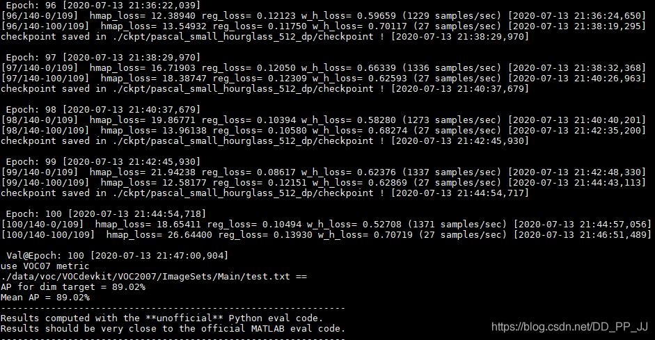
每隔5个epoch将进行一次eval,在自己的数据集上最终可以得到90%左右的mAP。
笔者将已经改好的单类的CenterNet放在Github上:https://github.com/pprp/SimpleCVReproduction/tree/master/CenterNet
5. 参考
[1]https://github.com/pprp/SimpleCVReproduction/tree/master/CenterNet
[2]https://github.com/zzzxxxttt/pytorch_simple_CenterNet_45
二、数据集加载过程
本章主要解读CenterNet如何加载数据,并将标注信息转化为CenterNet规定的高斯分布的形式。
1. YOLOv3和CenterNet流程对比
CenterNet和Anchor-Based的方法不同,以YOLOv3为例,大致梳理一下模型的框架和数据处理流程。
YOLOv3是一个经典的单阶段的目标检测算法,图片进入网络的流程如下:
- 对图片进行resize,长和宽都要是32的倍数。
- 图片经过网络的特征提取后,空间分辨率变为原来的1/32。
- 得到的Tensor去代表图片不同尺度下的目标框,其中目标框的表示为(x,y,w,h,c),分别代表左上角坐标,宽和高,含有某物体的置信度。
- 训练完成后,测试的时候需要使用非极大抑制算法得到最终的目标框。
CenterNet是一个经典的Anchor-Free目标检测方法,图片进入网络流程如下:
- 对图片进行resize,长和宽一般相等,并且至少为4的倍数。
- 图片经过网络的特征提取后,得到的特征图的空间分辨率依然比较大,是原来的¼。这是因为CenterNet采用的是类似人体姿态估计中用到的骨干网络,基于heatmap提取关键点的方法需要最终的空间分辨率比较大。
- 训练的过程中,CenterNet得到的是一个heatmap,所以标签加载的时候,需要转为类似的heatmap热图。
- 测试的过程中,由于只需要从热图中提取目标,这样就不需要使用NMS,降低了计算量。
2. CenterNet部分详解
设输入图片为I\in R^{W\times H\times 3}, W代表图片的宽,H代表高。CenterNet的输出是一个关键点热图heatmap。
其中R代表输出的stride大小,C代表关键点的类型的个数。
举个例子,在COCO数据集目标检测中,R设置为4,C的值为80,代表80个类别。
如果\hat{Y}_{x,y,c}=1代表检测到一个物体,表示对类别c来说,(x,y)这个位置检测到了c类的目标。
既然输出是热图,标签构建的ground truth也必须是热图的形式。标注的内容一般包含(x1,y1,x2,y2,c),目标框左上角坐标、右下角坐标和类别c,按照以下流程转为ground truth:
- 得到原图中对应的中心坐标p=(\frac{x1+x2}{2}, \frac{y1+y2}{2})
- 得到下采样后的feature map中对应的中心坐标\tilde{p}=\lfloor \frac{p}{R}\rfloor, R代表下采样倍数,CenterNet中R为4
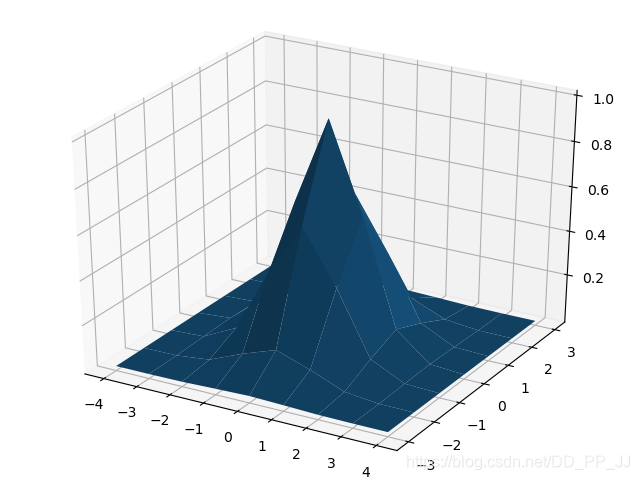
- 如果输入图片为512,那么输出的feature map的空间分辨率为[128x128], 将标注的目标框以高斯核的方式将关键点分布到特征图上:
其中\sigma_p是一个与目标大小相关的标准差(代码中设置的是)。对于特殊情况,相同类别的两个高斯分布发生了重叠,重叠元素间最大的值作为最终元素。下图是知乎用户OLDPAN分享的高斯分布图。
3. 代码部分
datasets/pascal.py 的代码主要从getitem函数入手,以下代码已经做了注释,其中最重要的两个部分一个是如何获取高斯半径(gaussian_radius函数),一个是如何将高斯分布分散到heatmap上(draw_umich_gaussian函数)。
def __getitem__(self, index):
    img_id = self.images[index]
    img_path = os.path.join(
        self.img_dir, self.coco.loadImgs(ids=[img_id])[0]['file_name'])
    ann_ids = self.coco.getAnnIds(imgIds=[img_id])
    annotations = self.coco.loadAnns(ids=ann_ids)

    labels = np.array([self.cat_ids[anno['category_id']]
                        for anno in annotations])
    bboxes = np.array([anno['bbox']
                        for anno in annotations], dtype=np.float32)

    if len(bboxes) == 0:
        bboxes = np.array([[0., 0., 0., 0.]], dtype=np.float32)
        labels = np.array([[0]])

    bboxes[:, 2:] += bboxes[:, :2]  # xywh to xyxy

    img = cv2.imread(img_path)
    height, width = img.shape[0], img.shape[1]
    # 获取中心坐标p
    center = np.array([width / 2., height / 2.],
                        dtype=np.float32)  # center of image
    scale = max(height, width) * 1.0  # 仿射变换

    flipped = False
    if self.split == 'train':
        # 随机选择一个尺寸来训练
        scale = scale * np.random.choice(self.rand_scales)
        w_border = get_border(128, width)
        h_border = get_border(128, height)
        center[0] = np.random.randint(low=w_border, high=width - w_border)
        center[1] = np.random.randint(low=h_border, high=height - h_border)

        if np.random.random() < 0.5:
            flipped = True
            img = img[:, ::-1, :]
            center[0] = width - center[0] - 1

    # 仿射变换
    trans_img = get_affine_transform(
        center, scale, 0, [self.img_size['w'], self.img_size['h']])
    img = cv2.warpAffine(
        img, trans_img, (self.img_size['w'], self.img_size['h']))

    # 归一化
    img = (img.astype(np.float32) / 255.)
    if self.split == 'train':
        # 对图片的亮度对比度等属性进行修改
        color_aug(self.data_rng, img, self.eig_val, self.eig_vec)

    img -= self.mean
    img /= self.std
    img = img.transpose(2, 0, 1)  # from [H, W, C] to [C, H, W]

    # 对Ground Truth heatmap进行仿射变换
    trans_fmap = get_affine_transform(
        center, scale, 0, [self.fmap_size['w'], self.fmap_size['h']]) # 这时候已经是下采样为原来的四分之一了

    # 3个最重要的变量
    hmap = np.zeros(
        (self.num_classes, self.fmap_size['h'], self.fmap_size['w']), dtype=np.float32)  # heatmap
    w_h_ = np.zeros((self.max_objs, 2), dtype=np.float32)  # width and height
    regs = np.zeros((self.max_objs, 2), dtype=np.float32)  # regression

    # indexs
    inds = np.zeros((self.max_objs,), dtype=np.int64)
    # 具体选择哪些index
    ind_masks = np.zeros((self.max_objs,), dtype=np.uint8)

    for k, (bbox, label) in enumerate(zip(bboxes, labels)):
        if flipped:
            bbox[[0, 2]] = width - bbox[[2, 0]] - 1

        # 对检测框也进行仿射变换
        bbox[:2] = affine_transform(bbox[:2], trans_fmap)
        bbox[2:] = affine_transform(bbox[2:], trans_fmap)
        # 防止越界
        bbox[[0, 2]] = np.clip(bbox[[0, 2]], 0, self.fmap_size['w'] - 1)
        bbox[[1, 3]] = np.clip(bbox[[1, 3]], 0, self.fmap_size['h'] - 1)
        # 得到高和宽
        h, w = bbox[3] - bbox[1], bbox[2] - bbox[0]

        if h > 0 and w > 0:
            obj_c = np.array([(bbox[0] + bbox[2]) / 2, (bbox[1] + bbox[3]) / 2],
                                dtype=np.float32) # 中心坐标-浮点型
            obj_c_int = obj_c.astype(np.int32) # 整型的中心坐标
            # 根据一元二次方程计算出最小的半径
            radius = max(0, int(gaussian_radius((math.ceil(h), math.ceil(w)), self.gaussian_iou)))
            # 得到高斯分布
            draw_umich_gaussian(hmap[label], obj_c_int, radius)

            w_h_[k] = 1. * w, 1. * h

            # 记录偏移量
            regs[k] = obj_c - obj_c_int  # discretization error
            # 当前是obj序列中的第k个 = fmap_w * cy + cx = fmap中的序列数
            inds[k] = obj_c_int[1] * self.fmap_size['w'] + obj_c_int[0]
            # 进行mask标记
            ind_masks[k] = 1

    return {'image': img, 'hmap': hmap, 'w_h_': w_h_, 'regs': regs,
            'inds': inds, 'ind_masks': ind_masks, 'c': center,
            's': scale, 'img_id': img_id}
4. heatmap上应用高斯核
heatmap上使用高斯核有很多需要注意的细节。CenterNet官方版本实际上是在CornerNet的基础上改动得到的,有很多祖传代码。
在使用高斯核前要考虑这样一个问题,下图来自于CornerNet论文中的图示,红色的是标注框,但绿色的其实也可以作为最终的检测结果保留下来。那么这个问题可以转化为绿框在红框多大范围以内可以被接受。使用IOU来衡量红框和绿框的贴合程度,当两者IOU>0.7的时候,认为绿框也可以被接受,反之则不被接受。
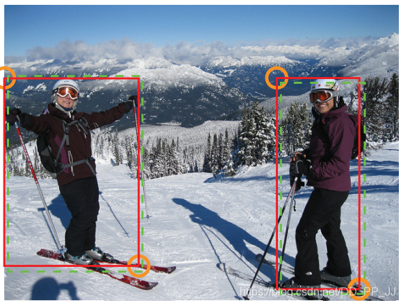
那么现在问题转化为,如何确定半径r, 让红框和绿框的IOU大于0.7。
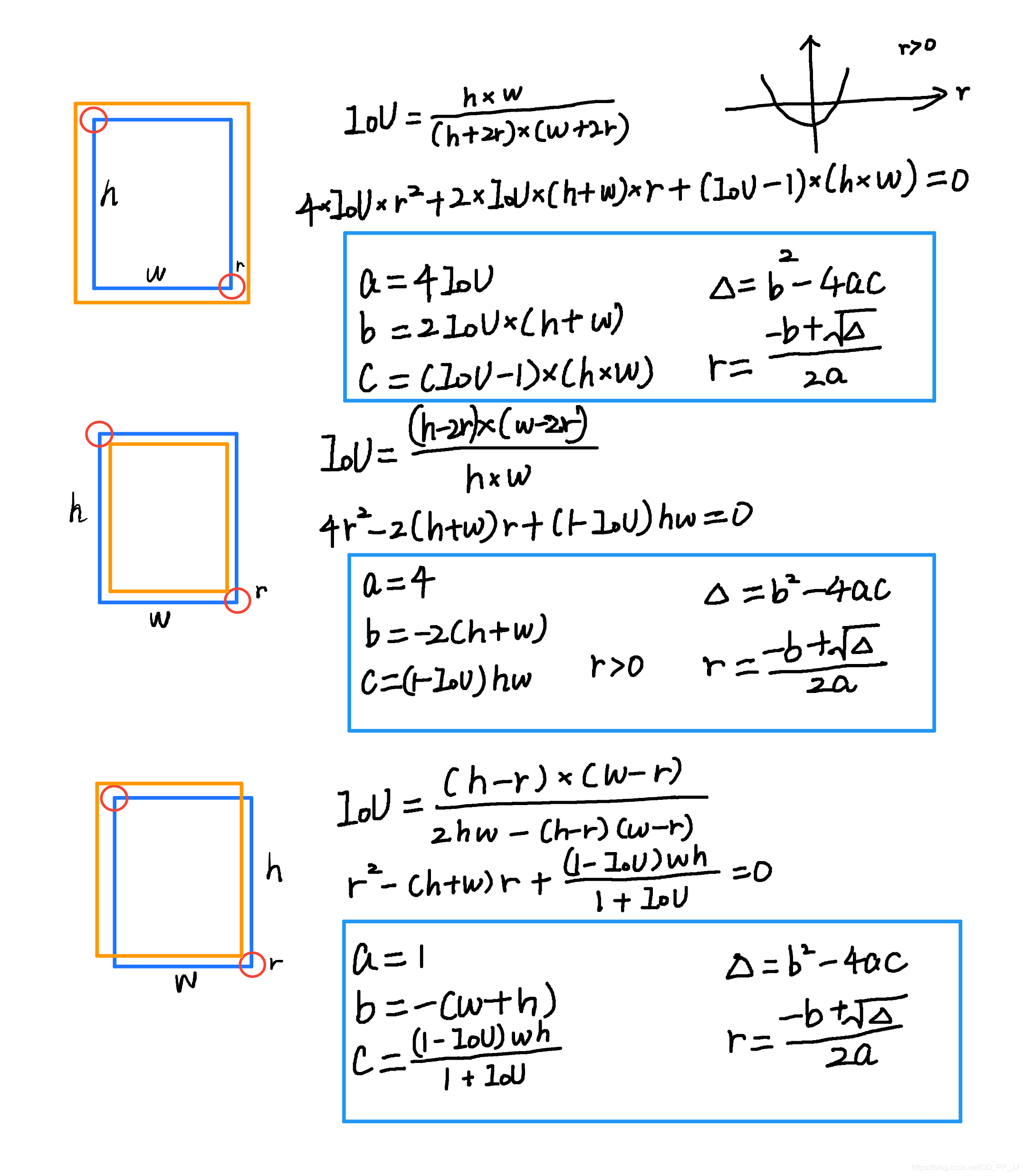
以上是三种情况,其中蓝框代表标注框,橙色代表可能满足要求的框。这个问题最终变为了一个一元二次方程有解的问题,同时由于半径必须为正数,所以r的取值就可以通过求根公式获得。
def gaussian_radius(det_size, min_overlap=0.7):
    # gt框的长和宽
    height, width = det_size

    a1 = 1
    b1 = (height + width)
    c1 = width * height * (1 - min_overlap) / (1 + min_overlap)
    sq1 = np.sqrt(b1 ** 2 - 4 * a1 * c1)
    r1 = (b1 + sq1) / (2 * a1)

    a2 = 4
    b2 = 2 * (height + width)
    c2 = (1 - min_overlap) * width * height
    sq2 = np.sqrt(b2 ** 2 - 4 * a2 * c2)
    r2 = (b2 + sq2) / (2 * a2)

    a3 = 4 * min_overlap
    b3 = -2 * min_overlap * (height + width)
    c3 = (min_overlap - 1) * width * height
    sq3 = np.sqrt(b3 ** 2 - 4 * a3 * c3)
    r3 = (b3 + sq3) / (2 * a3)

    return min(r1, r2, r3)
可以看到这里的公式和上图计算的结果是一致的,需要说明的是,CornerNet最开始版本中这里出现了错误,分母不是2a,而是直接设置为2。CenterNet也延续了这个bug,CenterNet作者回应说这个bug对结果的影响不大,但是根据issue的讨论来看,有一些人通过修正这个bug以后,可以让AR提升1-3个百分点。以下是有bug的版本,CornerNet最新版中已经修复了这个bug。
def gaussian_radius(det_size, min_overlap=0.7):
  height, width = det_size

  a1  = 1
  b1  = (height + width)
  c1  = width * height * (1 - min_overlap) / (1 + min_overlap)
  sq1 = np.sqrt(b1 ** 2 - 4 * a1 * c1)
  r1  = (b1 + sq1) / 2

  a2  = 4
  b2  = 2 * (height + width)
  c2  = (1 - min_overlap) * width * height
  sq2 = np.sqrt(b2 ** 2 - 4 * a2 * c2)
  r2  = (b2 + sq2) / 2

  a3  = 4 * min_overlap
  b3  = -2 * min_overlap * (height + width)
  c3  = (min_overlap - 1) * width * height
  sq3 = np.sqrt(b3 ** 2 - 4 * a3 * c3)
  r3  = (b3 + sq3) / 2

  return min(r1, r2, r3)
同时有一些人认为圆并不普适,提出了使用椭圆来进行计算,也有人在issue中给出了推导,感兴趣的可以看以下链接:https://github.com/princeton-vl/CornerNet/issues/110
5. 高斯分布添加到heatmap上
def gaussian2D(shape, sigma=1):
    m, n = [(ss - 1.) / 2. for ss in shape]
    y, x = np.ogrid[-m:m + 1, -n:n + 1]

    h = np.exp(-(x * x + y * y) / (2 * sigma * sigma))
    h[h < np.finfo(h.dtype).eps * h.max()] = 0
    # 限制最小的值
    return h

def draw_umich_gaussian(heatmap, center, radius, k=1):
    # 得到直径
    diameter = 2 * radius + 1
    gaussian = gaussian2D((diameter, diameter), sigma=diameter / 6)
    # sigma是一个与直径相关的参数
    # 一个圆对应内切正方形的高斯分布

    x, y = int(center[0]), int(center[1])

    height, width = heatmap.shape[0:2]

    # 对边界进行约束,防止越界
    left, right = min(x, radius), min(width - x, radius + 1)
    top, bottom = min(y, radius), min(height - y, radius + 1)

    # 选择对应区域
    masked_heatmap = heatmap[y - top:y + bottom, x - left:x + right]
    # 将高斯分布结果约束在边界内
    masked_gaussian = gaussian[radius - top:radius + bottom,
                               radius - left:radius + right]

    if min(masked_gaussian.shape) > 0 and min(masked_heatmap.shape) > 0:  # TODO debug
        np.maximum(masked_heatmap, masked_gaussian * k, out=masked_heatmap)
        # 将高斯分布覆盖到heatmap上,相当于不断的在heatmap基础上添加关键点的高斯,
        # 即同一种类型的框会在一个heatmap某一个类别通道上面上面不断添加。
        # 最终通过函数总体的for循环,相当于不断将目标画到heatmap
    return heatmap
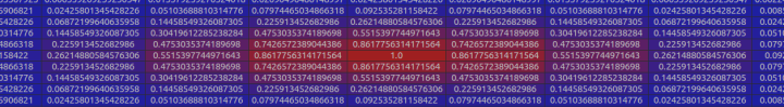
使用matplotlib对gaussian2D进行可视化。
import numpy as np
y,x = np.ogrid[-4:5,-3:4]
sigma = 1
h=np.exp(-(x*x+y*y)/(2*sigma*sigma))
import matplotlib.pyplot as plt
from mpl_toolkits.mplot3d import Axes3D
fig = plt.figure()
ax = Axes3D(fig)
ax.plot_surface(x,y,h)
plt.show()
6. 参考
[1]https://zhuanlan.zhihu.com/p/66048276
[2]https://www.cnblogs.com/shine-lee/p/9671253.html
[3]https://zhuanlan.zhihu.com/p/96856635
[4]http://xxx.itp.ac.cn/pdf/1808.01244
[5]https://github.com/princeton-vl/CornerNet/issues/110
三、骨干网络之hourglass
CenterNet中主要提供了三个骨干网络ResNet-18(ResNet-101), DLA-34, Hourglass-104,本章从结构和代码先对hourglass进行讲解。
1. Ground Truth Heatmap
在开始讲解骨干网络之前,先提一下上一篇文章中有朋友问我的问题:CenterNet为什么要沿用CornerNet的半径计算方式?
查询了CenterNet论文还有官方实现的issue,其实没有明确指出为何要用CornerNet的半径,issue中回复也说是这是沿用了CornerNet的祖传代码。经过和@tangsipeng的讨论,讨论结果如下:
以下代码是涉及到半径计算的部分:
# 根据一元二次方程计算出最小的半径
radius = max(0, int(gaussian_radius((math.ceil(h), math.ceil(w)), self.gaussian_iou)))
# 得到高斯分布
draw_umich_gaussian(hmap[label], obj_c_int, radius)
在centerNet中,半径的存在主要是用于计算高斯分布的sigma值,而这个值也是一个经验性判定结果。
def draw_umich_gaussian(heatmap, center, radius, k=1):
    # 得到直径
    diameter = 2 * radius + 1
    gaussian = gaussian2D((diameter, diameter), sigma=diameter / 6)
    # 一个圆对应内切正方形的高斯分布

    x, y = int(center[0]), int(center[1])

    height, width = heatmap.shape[0:2]

    # 对边界进行约束,防止越界
    left, right = min(x, radius), min(width - x, radius + 1)
    top, bottom = min(y, radius), min(height - y, radius + 1)

    # 选择对应区域
    masked_heatmap = heatmap[y - top:y + bottom, x - left:x + right]
    # 将高斯分布结果约束在边界内
    masked_gaussian = gaussian[radius - top:radius + bottom,
                               radius - left:radius + right]

    if min(masked_gaussian.shape) > 0 and min(masked_heatmap.shape) > 0:
        np.maximum(masked_heatmap, masked_gaussian * k, out=masked_heatmap)
        # 将高斯分布覆盖到heatmap上,相当于不断的在heatmap基础上添加关键点的高斯,
        # 即同一种类型的框会在一个heatmap某一个类别通道上面上面不断添加。
        # 最终通过函数总体的for循环,相当于不断将目标画到heatmap
    return heatmap
合理推测一下(不喜勿喷),之前很多人在知乎上issue里讨论这个半径计算的时候,有提到这样的问题,就是如果将CenterNet对应的2a改正确了,反而效果会差。
我觉得这个问题可能和这里的sigma=diameter / 6有一定的关系,作者当时用祖传代码(2a那部分有错)进行调参,然后确定了sigma。这时这个sigma就和祖传代码是对应的,如果修改了祖传代码,同样也需要改一下sigma或者调一下参数。
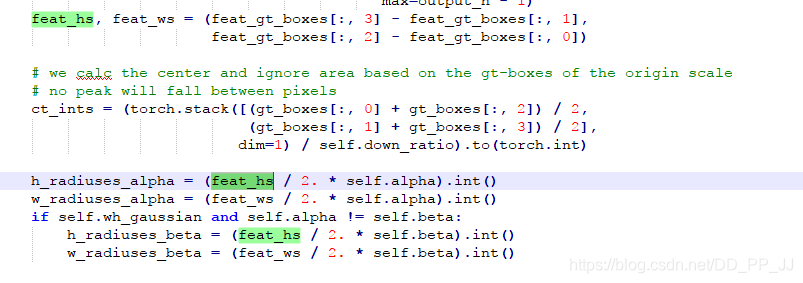
tangsipeng同学分享的文章《Training-Time-Friendly Network for Real-Time Object Detection》对应计算高斯核sigma部分就没有用cornernet的祖传代码,对应代码可以发现,这里的sigma是一个和h,w相关的超参数,也是手工挑选的。
综上,目前暂时认为CenterNet直接沿用CornerNet的祖传代码没有官方的解释,我们也暂时没有想到解释。如果对这个问题有研究的同学欢迎联系笔者。
2. Hourglass
Hourglass网络结构最初是在ECCV2016的Stacked hourglass networks for human pose estimation文章中提出的,用于人体姿态估计。Stacked Hourglass就是把多个漏斗形状的网络级联起来,可以获取多尺度的信息。
Hourglass的设计比较有层次,通过各个模块的有规律组合成完整网络。
2.1 Residual模块
class residual(nn.Module):
    def __init__(self, k, inp_dim, out_dim, stride=1, with_bn=True):
        super(residual, self).__init__()

        self.conv1 = nn.Conv2d(inp_dim,
                               out_dim, (3, 3),
                               padding=(1, 1),
                               stride=(stride, stride),
                               bias=False)
        self.bn1 = nn.BatchNorm2d(out_dim)
        self.relu1 = nn.ReLU(inplace=True)

        self.conv2 = nn.Conv2d(out_dim,
                               out_dim, (3, 3),
                               padding=(1, 1),
                               bias=False)
        self.bn2 = nn.BatchNorm2d(out_dim)

        self.skip = nn.Sequential(nn.Conv2d(inp_dim, out_dim, (1, 1), stride=(stride, stride), bias=False),
                                  nn.BatchNorm2d(out_dim)) \
            if stride != 1 or inp_dim != out_dim else nn.Sequential()
        self.relu = nn.ReLU(inplace=True)

    def forward(self, x):
        conv1 = self.conv1(x)
        bn1 = self.bn1(conv1)
        relu1 = self.relu1(bn1)

        conv2 = self.conv2(relu1)
        bn2 = self.bn2(conv2)

        skip = self.skip(x)
        return self.relu(bn2 + skip)
就是简单的残差链接网络中的最基础的残差模块。
2.2 Hourglass子模块
class kp_module(nn.Module):
    '''
    kp module指的是hourglass基本模块
    '''
    def __init__(self, n, dims, modules):
        super(kp_module, self).__init__()

        self.n = n

        curr_modules = modules[0]
        next_modules = modules[1]

        curr_dim = dims[0]
        next_dim = dims[1]

        # curr_mod x residual,curr_dim -> curr_dim -> ... -> curr_dim
        self.top = make_layer(3, # 空间分辨率不变
                              curr_dim,
                              curr_dim,
                              curr_modules,
                              layer=residual)
        self.down = nn.Sequential() # 暂时没用
        # curr_mod x residual,curr_dim -> next_dim -> ... -> next_dim
        self.low1 = make_layer(3,
                               curr_dim,
                               next_dim,
                               curr_modules,
                               layer=residual,
                               stride=2)# 降维
        # next_mod x residual,next_dim -> next_dim -> ... -> next_dim
        if self.n > 1:
            # 通过递归完成构建
            self.low2 = kp_module(n - 1, dims[1:], modules[1:])
        else:
            # 递归出口
            self.low2 = make_layer(3,
                                   next_dim,
                                   next_dim,
                                   next_modules,
                                   layer=residual)
        # curr_mod x residual,next_dim -> next_dim -> ... -> next_dim -> curr_dim
        self.low3 = make_layer_revr(3, # 升维
                                    next_dim,
                                    curr_dim,
                                    curr_modules,
                                    layer=residual)
        self.up = nn.Upsample(scale_factor=2) # 上采样进行升维

    def forward(self, x):
        up1 = self.top(x)
        down = self.down(x)
        low1 = self.low1(down)
        low2 = self.low2(low1)
        low3 = self.low3(low2)
        up2 = self.up(low3)
        return up1 + up2
其中有两个主要的函数make_layer和make_layer_revr,make_layer将空间分辨率降维,make_layer_revr函数进行升维,所以将这个结构命名为hourglass(沙漏)。
核心构建是一个递归函数,递归层数是通过n来控制,称之为n阶hourglass模块。
2.3 Hourglass
class exkp(nn.Module):
    '''
     整体模型调用
     large hourglass stack为2
     small hourglass stack为1
     n这里控制的是hourglass的阶数,以上两个都用的是5阶的hourglass
     exkp(n=5, nstack=2, dims=[256, 256, 384, 384, 384, 512], modules=[2, 2, 2, 2, 2, 4]),
    '''
    def __init__(self, n, nstack, dims, modules, cnv_dim=256, num_classes=80):
        super(exkp, self).__init__()

        self.nstack = nstack # 堆叠多次hourglass
        self.num_classes = num_classes

        curr_dim = dims[0]

        # 快速降维为原来的1/4
        self.pre = nn.Sequential(convolution(7, 3, 128, stride=2),
                                 residual(3, 128, curr_dim, stride=2))

        # 堆叠nstack个hourglass
        self.kps = nn.ModuleList(
            [kp_module(n, dims, modules) for _ in range(nstack)])

        self.cnvs = nn.ModuleList(
            [convolution(3, curr_dim, cnv_dim) for _ in range(nstack)])

        self.inters = nn.ModuleList(
            [residual(3, curr_dim, curr_dim) for _ in range(nstack - 1)])

        self.inters_ = nn.ModuleList([
            nn.Sequential(nn.Conv2d(curr_dim, curr_dim, (1, 1), bias=False),
                          nn.BatchNorm2d(curr_dim)) for _ in range(nstack - 1)
        ])
        self.cnvs_ = nn.ModuleList([
            nn.Sequential(nn.Conv2d(cnv_dim, curr_dim, (1, 1), bias=False),
                          nn.BatchNorm2d(curr_dim)) for _ in range(nstack - 1)
        ])
        # heatmap layers
        self.hmap = nn.ModuleList([
            make_kp_layer(cnv_dim, curr_dim, num_classes) # heatmap输出通道为num_classes
            for _ in range(nstack)
        ])
        for hmap in self.hmap:
            # -2.19是focal loss中的默认参数,论文的4.1节有详细说明,-ln((1-pi)/pi),这里的pi取0.1
            hmap[-1].bias.data.fill_(-2.19)

        # regression layers
        self.regs = nn.ModuleList(
            [make_kp_layer(cnv_dim, curr_dim, 2) for _ in range(nstack)]) # 回归的输出通道为2
        self.w_h_ = nn.ModuleList(
            [make_kp_layer(cnv_dim, curr_dim, 2) for _ in range(nstack)]) # wh

        self.relu = nn.ReLU(inplace=True)

    def forward(self, image):
        inter = self.pre(image)

        outs = []
        for ind in range(self.nstack): # 堆叠两次hourglass
            kp = self.kps[ind](inter)
            cnv = self.cnvs[ind](kp)

            if self.training or ind == self.nstack - 1:
                outs.append([
                    self.hmap[ind](cnv), self.regs[ind](cnv),
                    self.w_h_[ind](cnv)
                ])

            if ind < self.nstack - 1:
                inter = self.inters_[ind](inter) + self.cnvs_[ind](cnv)
                inter = self.relu(inter)
                inter = self.inters[ind](inter)
        return outs
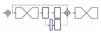
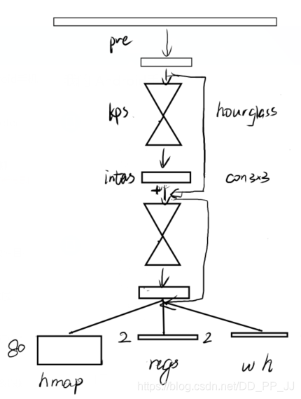
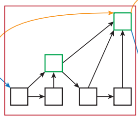
这里需要注意的是inters变量,这个变量保存的是中间监督过程,可以在这个位置添加loss,具体如下图蓝色部分所示,在这个部分可以添加loss,然后再用1x1卷积重新映射到对应的通道个数并相加。
然后再来谈三个输出,假设当前是COCO数据集,类别个数为80,那么hmap相当于输出了通道个数为80的heatmap,每个通道负责预测一个类别;wh代表对应中心点的宽和高;regs是偏置量。
CenterNet论文详解可以点击【目标检测Anchor-Free】CVPR 2019 Object as Points(CenterNet)
整个网络就梳理完成了,笔者简单画了一下nstack为2时的hourglass网络,如下图所示:
3. Reference
[1]https://blog.csdn.net/shenxiaolu1984/article/details/51428392
[2]http://xxx.itp.ac.cn/pdf/1603.06937.pdf
[3]http://xxx.itp.ac.cn/pdf/1904.07850v1
四、骨干网络之DLASeg
DLA全称是Deep Layer Aggregation, 于2018年发表于CVPR。被CenterNet, FairMOT等框架所采用,其效果很不错,准确率和模型复杂度平衡的也比较好。
CenterNet中使用的DLASeg是在DLA-34的基础上添加了Deformable Convolution后的分割网络。
1. 简介
Aggretation聚合是目前设计网络结构的常用的一种技术。如何将不同深度,将不同stage、block之间的信息进行融合是本文探索的目标。
目前常见的聚合方式有skip connection, 如ResNet,这种融合方式仅限于块内部,并且融合方式仅限于简单的叠加。
本文提出了DLA的结构,能够迭代式地将网络结构的特征信息融合起来,让模型有更高的精度和更少的参数。
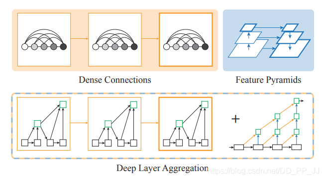
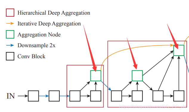
上图展示了DLA的设计思路,Dense Connections来自DenseNet,可以聚合语义信息。Feature Pyramids空间特征金字塔可以聚合空间信息。DLA则是将两者更好地结合起来从而可以更好的获取what和where的信息。仔细看一下DLA的其中一个模块,如下图所示:
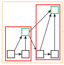
研读过代码以后,可以看出这个花里胡哨的结构其实是按照树的结构进行组织的,红框框住的就是两个树,树之间又采用了类似ResNet的残差链接结构。
2. 核心
先来重新梳理一下上边提到的语义信息和空间信息,文章给出了详细解释:
- 语义融合:在通道方向进行的聚合,能够提高模型推断“是什么”的能力(what)
- 空间融合:在分辨率和尺度方向的融合,能够提高模型推断“在哪里”的能力(where)
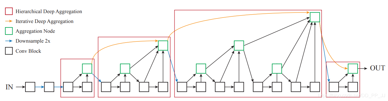
Deep Layer Aggregation核心模块有两个IDA(Iterative Deep Aggregation)和HDA(Hierarchical Deep Aggregation),如上图所示。
-
红色框代表的是用树结构链接的层次结构,能够更好地传播特征和梯度。
-
黄色链接代表的是IDA,负责链接相邻两个stage的特征让深层和浅层的表达能更好地融合。
- 蓝色连线代表进行了下采样,网络一开始也和ResNet一样进行了快速下采样。
论文中也给了公式推导,感兴趣的可以去理解一下。本章还是将重点放在代码实现上。
3. 实现
这部分代码复制自CenterNet官方实现,https://github.com/pprp/SimpleCVReproduction/blob/master/CenterNet/nets/dla34.py
3.1 基础模块
首先是三个模块,BasicBlock和Bottleneck和ResNet中的一致,BottleneckX实际上是ResNeXt中的基础模块,也可以作为DLA中的基础模块。DLA34中调用的依然是BasicBlock。
class BasicBlock(nn.Module):
    def __init__(self, inplanes, planes, stride=1, dilation=1):
        super(BasicBlock, self).__init__()
        self.conv1 = nn.Conv2d(inplanes, planes, kernel_size=3,
                               stride=stride, padding=dilation,
                               bias=False, dilation=dilation)
        self.bn1 = BatchNorm(planes)
        self.relu = nn.ReLU(inplace=True)
        self.conv2 = nn.Conv2d(planes, planes, kernel_size=3,
                               stride=1, padding=dilation,
                               bias=False, dilation=dilation)
        self.bn2 = BatchNorm(planes)
        self.stride = stride

    def forward(self, x, residual=None):
        if residual is None:
            residual = x
        out = self.conv1(x)
        out = self.bn1(out)
        out = self.relu(out)
        out = self.conv2(out)
        out = self.bn2(out)
        out += residual
        out = self.relu(out)
        return out


class Bottleneck(nn.Module):
    expansion = 2
    def __init__(self, inplanes, planes, stride=1, dilation=1):
        super(Bottleneck, self).__init__()
        expansion = Bottleneck.expansion
        bottle_planes = planes // expansion
        self.conv1 = nn.Conv2d(inplanes, bottle_planes,
                               kernel_size=1, bias=False)
        self.bn1 = BatchNorm(bottle_planes)
        self.conv2 = nn.Conv2d(bottle_planes, bottle_planes, kernel_size=3,
                               stride=stride, padding=dilation,
                               bias=False, dilation=dilation)
        self.bn2 = BatchNorm(bottle_planes)
        self.conv3 = nn.Conv2d(bottle_planes, planes,
                               kernel_size=1, bias=False)
        self.bn3 = BatchNorm(planes)
        self.relu = nn.ReLU(inplace=True)
        self.stride = stride

    def forward(self, x, residual=None):
        if residual is None:
            residual = x
        out = self.conv1(x)
        out = self.bn1(out)
        out = self.relu(out)
        out = self.conv2(out)
        out = self.bn2(out)
        out = self.relu(out)
        out = self.conv3(out)
        out = self.bn3(out)
        out += residual
        out = self.relu(out)
        return out

class BottleneckX(nn.Module):
    expansion = 2
    cardinality = 32
    def __init__(self, inplanes, planes, stride=1, dilation=1):
        super(BottleneckX, self).__init__()
        cardinality = BottleneckX.cardinality
        # dim = int(math.floor(planes * (BottleneckV5.expansion / 64.0)))
        # bottle_planes = dim * cardinality
        bottle_planes = planes * cardinality // 32
        self.conv1 = nn.Conv2d(inplanes, bottle_planes,
                               kernel_size=1, bias=False)
        self.bn1 = BatchNorm(bottle_planes)
        self.conv2 = nn.Conv2d(bottle_planes, bottle_planes, kernel_size=3,
                               stride=stride, padding=dilation, bias=False,
                               dilation=dilation, groups=cardinality)
        self.bn2 = BatchNorm(bottle_planes)
        self.conv3 = nn.Conv2d(bottle_planes, planes,
                               kernel_size=1, bias=False)
        self.bn3 = BatchNorm(planes)
        self.relu = nn.ReLU(inplace=True)
        self.stride = stride

    def forward(self, x, residual=None):
        if residual is None:
            residual = x
        out = self.conv1(x)
        out = self.bn1(out)
        out = self.relu(out)
        out = self.conv2(out)
        out = self.bn2(out)
        out = self.relu(out)
        out = self.conv3(out)
        out = self.bn3(out)
        out += residual
        out = self.relu(out)
        return out
3.2 Root类
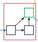
然后就是Root类,对应下图中的绿色模块
所有的Aggregation Node都是通过调用这个模块完成的,这个绿色结点也是其连接两个树的根,所以形象地称之为Root。下面是代码实现,forward函数中接受的是多个对象,用来聚合多个层的信息。
class Root(nn.Module):
    def __init__(self, in_channels, out_channels, kernel_size, residual):
        super(Root, self).__init__()
        self.conv = nn.Conv2d(
            in_channels, out_channels, 1,
            stride=1, bias=False, padding=(kernel_size - 1) // 2)
        self.bn = BatchNorm(out_channels)
        self.relu = nn.ReLU(inplace=True)
        self.residual = residual

    def forward(self, *x):
        # 输入是多个层输出结果
        children = x
        x = self.conv(torch.cat(x, 1))
        x = self.bn(x)
        if self.residual:
            x += children[0]
        x = self.relu(x)

        return x
3.3 Tree类
Tree类对应图中的HDA模块,是最核心最复杂的地方,建议手动画一下。其核心就是递归调用的Tree类的构建,以下是代码。
class Tree(nn.Module):
    '''
    self.level5 = Tree(levels[5], block, channels[4], channels[5], 2,
                    level_root=True, root_residual=residual_root)
    '''
    def __init__(self, levels, block, in_channels, out_channels, stride=1,
                 level_root=False, root_dim=0, root_kernel_size=1,
                 dilation=1, root_residual=False):
        super(Tree, self).__init__()
        if root_dim == 0:
            root_dim = 2 * out_channels
        if level_root:
            root_dim += in_channels
        if levels == 1:
            self.tree1 = block(in_channels, out_channels, stride,
                               dilation=dilation)
            self.tree2 = block(out_channels, out_channels, 1,
                               dilation=dilation)
        else:
            self.tree1 = Tree(levels - 1, block, in_channels, out_channels,
                              stride, root_dim=0,
                              root_kernel_size=root_kernel_size,
                              dilation=dilation, root_residual=root_residual)
            self.tree2 = Tree(levels - 1, block, out_channels, out_channels,
                              root_dim=root_dim + out_channels,
                              root_kernel_size=root_kernel_size,
                              dilation=dilation, root_residual=root_residual)
        if levels == 1:
            self.root = Root(root_dim, out_channels, root_kernel_size,
                             root_residual)
        self.level_root = level_root
        self.root_dim = root_dim
        self.downsample = None
        self.project = None
        self.levels = levels
        if stride > 1:
            self.downsample = nn.MaxPool2d(stride, stride=stride)
        if in_channels != out_channels:
            self.project = nn.Sequential(
                nn.Conv2d(in_channels, out_channels,
                          kernel_size=1, stride=1, bias=False),
                BatchNorm(out_channels)
            )

    def forward(self, x, residual=None, children=None):
        children = [] if children is None else children

        bottom = self.downsample(x) if self.downsample else x
        # project就是映射,如果输入输出通道数不同则将输入通道数映射到输出通道数
        residual = self.project(bottom) if self.project else bottom

        if self.level_root:
            children.append(bottom)

        x1 = self.tree1(x, residual)
        if self.levels == 1:
            x2 = self.tree2(x1)
            # root是出口
            x = self.root(x2, x1, *children)
        else:
            children.append(x1)
            x = self.tree2(x1, children=children)
        return x
经过笔者研究,这里涉及了两个比较重要的参数level和level root。
这个类有两个重要的成员变量tree1和tree2,是通过递归的方式迭代生成的,迭代层数通过level进行控制的,举两个例子,第一个是level为1,并且level root=True的情况,对照代码和下图可以理解得到:
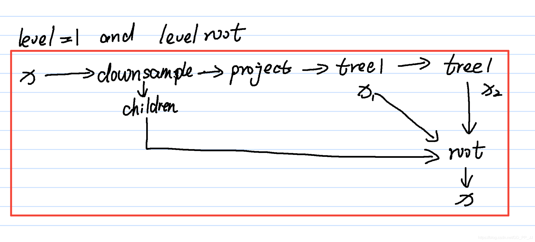
也就是对应的是:
代码中的children参数是一个list,保存的是所有传给Root的成员,这些成员将作为其中的叶子结点。
第二个例子是level=2, level root=True的情况,如下图所示:
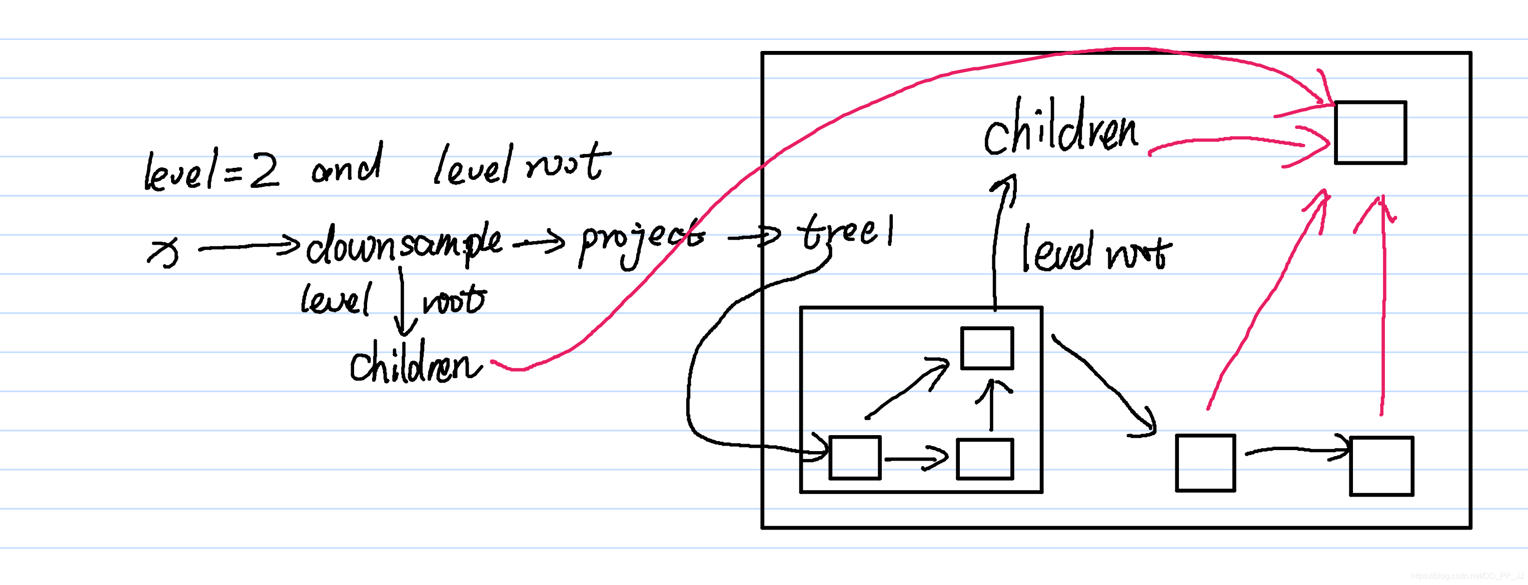
这部分代码对应的是:
粉色箭头是children对象,都交给Root进行聚合操作。
3.4 DLA
Tree是DLA最重要的模块,Tree搞定之后,DLA就按顺序拼装即可。
class DLA(nn.Module):
    '''
    DLA([1, 1, 1, 2, 2, 1],
        [16, 32, 64, 128, 256, 512],
        block=BasicBlock, **kwargs)
    '''
    def __init__(self, levels, channels, num_classes=1000,
                 block=BasicBlock, residual_root=False, return_levels=False,
                 pool_size=7, linear_root=False):
        super(DLA, self).__init__()
        self.channels = channels
        self.return_levels = return_levels
        self.num_classes = num_classes
        self.base_layer = nn.Sequential(
            nn.Conv2d(3, channels[0], kernel_size=7, stride=1,
                      padding=3, bias=False),
            BatchNorm(channels[0]),
            nn.ReLU(inplace=True))
        # 在最初前两层仅仅使用卷积层
        self.level0 = self._make_conv_level(
            channels[0], channels[0], levels[0])
        self.level1 = self._make_conv_level(
            channels[0], channels[1], levels[1], stride=2)
        '''
        if level_root:
            root_dim += in_channels
        '''
        self.level2 = Tree(levels[2], block, channels[1], channels[2], 2,
                           level_root=False, root_residual=residual_root)
        self.level3 = Tree(levels[3], block, channels[2], channels[3], 2,
                           level_root=True, root_residual=residual_root)
        self.level4 = Tree(levels[4], block, channels[3], channels[4], 2,
                           level_root=True, root_residual=residual_root)
        self.level5 = Tree(levels[5], block, channels[4], channels[5], 2,
                           level_root=True, root_residual=residual_root)

        self.avgpool = nn.AvgPool2d(pool_size)
        self.fc = nn.Conv2d(channels[-1], num_classes, kernel_size=1,
                            stride=1, padding=0, bias=True)

        for m in self.modules():
            if isinstance(m, nn.Conv2d):
                n = m.kernel_size[0] * m.kernel_size[1] * m.out_channels
                m.weight.data.normal_(0, math.sqrt(2. / n))
            elif isinstance(m, BatchNorm):
                m.weight.data.fill_(1)
                m.bias.data.zero_()

    def forward(self, x):
        y = []
        x = self.base_layer(x)
        for i in range(6):
            # 将几个level串联起来
            x = getattr(self, 'level{}'.format(i))(x)
            y.append(x)
        if self.return_levels:
            return y
        else:
            x = self.avgpool(x)
            x = self.fc(x)
            x = x.view(x.size(0), -1)
            return x
4. DLASeg
DLASeg是在DLA的基础上使用Deformable Convolution和Upsample层组合进行信息提取,提升了空间分辨率。
class DLASeg(nn.Module):
    '''
    DLASeg('dla{}'.format(num_layers), heads,
                 pretrained=True,
                 down_ratio=down_ratio,
                 final_kernel=1,
                 last_level=5,
                 head_conv=head_conv)
    '''
    def __init__(self, base_name, heads, pretrained, down_ratio, final_kernel,
                 last_level, head_conv, out_channel=0):
        super(DLASeg, self).__init__()
        assert down_ratio in [2, 4, 8, 16]
        self.first_level = int(np.log2(down_ratio))
        self.last_level = last_level
        # globals() 函数会以字典类型返回当前位置的全部全局变量。
        # 所以这个base就相当于原来的DLA34
        self.base = globals()[base_name](pretrained=pretrained)
        channels = self.base.channels
        scales = [2 ** i for i in range(len(channels[self.first_level:]))]
        # first_level = 2 if down_ratio=4
        # channels = [16, 32, 64, 128, 256, 512] to [64, 128, 256, 512]
        # scales = [1, 2, 4, 8]
        self.dla_up = DLAUp(self.first_level, channels[self.first_level:], scales)

        if out_channel == 0:
            out_channel = channels[self.first_level]

        # 进行上采样
        self.ida_up = IDAUp(out_channel, channels[self.first_level:self.last_level],
                            [2 ** i for i in range(self.last_level - self.first_level)])

        self.heads = heads
        for head in self.heads:
            classes = self.heads[head]
            if head_conv > 0:
              fc = nn.Sequential(
                  nn.Conv2d(channels[self.first_level], head_conv,
                    kernel_size=3, padding=1, bias=True),
                  nn.ReLU(inplace=True),
                  nn.Conv2d(head_conv, classes,
                    kernel_size=final_kernel, stride=1,
                    padding=final_kernel // 2, bias=True))
              if 'hm' in head:
                fc[-1].bias.data.fill_(-2.19)
              else:
                fill_fc_weights(fc)
            else:
              fc = nn.Conv2d(channels[self.first_level], classes,
                  kernel_size=final_kernel, stride=1,
                  padding=final_kernel // 2, bias=True)
              if 'hm' in head:
                fc.bias.data.fill_(-2.19)
              else:
                fill_fc_weights(fc)
            self.__setattr__(head, fc)
    def forward(self, x):
        x = self.base(x)
        x = self.dla_up(x)
        y = []
        for i in range(self.last_level - self.first_level):
            y.append(x[i].clone())
        self.ida_up(y, 0, len(y))
        z = {}
        for head in self.heads:
            z[head] = self.__getattr__(head)(y[-1])
        return [z]
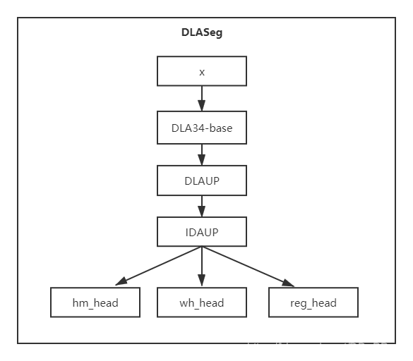
以上就是DLASeg的主要代码,其中负责上采样部分的是:
 self.ida_up = IDAUp(out_channel, channels[self.first_level:self.last_level],
[2 ** i for i in range(self.last_level - self.first_level)])
这部分负责解码,将空间分辨率提高。
class IDAUp(nn.Module):
    '''
    IDAUp(channels[j], in_channels[j:], scales[j:] // scales[j])
    ida(layers, len(layers) -i - 2, len(layers))
    '''
    def __init__(self, o, channels, up_f):
        super(IDAUp, self).__init__()
        for i in range(1, len(channels)):
            c = channels[i]
            f = int(up_f[i])
            proj = DeformConv(c, o)
            node = DeformConv(o, o)
            up = nn.ConvTranspose2d(o, o, f * 2, stride=f,
                                    padding=f // 2, output_padding=0,
                                    groups=o, bias=False)
            fill_up_weights(up)
            setattr(self, 'proj_' + str(i), proj)
            setattr(self, 'up_' + str(i), up)
            setattr(self, 'node_' + str(i), node)

    def forward(self, layers, startp, endp):
        for i in range(startp + 1, endp):
            upsample = getattr(self, 'up_' + str(i - startp))
            project = getattr(self, 'proj_' + str(i - startp))

            layers[i] = upsample(project(layers[i]))
            node = getattr(self, 'node_' + str(i - startp))
            layers[i] = node(layers[i] + layers[i - 1])
其核心是DLAUP和IDAUP, 这两个类中都使用了两个Deformable Convolution可变形卷积,然后使用ConvTranspose2d进行上采样,具体网络结构如下图所示。
5. 参考
[1]https://arxiv.org/abs/1707.06484
[2]https://github.com/pprp/SimpleCVReproduction/blob/master/CenterNet/nets/dla34.py
五、CenterNet Loss详解
本章主要讲解CenterNet的loss,由偏置部分(reg loss)、热图部分(heatmap loss)、宽高(wh loss)部分三部分loss组成,附代码实现。
1. 网络输出
论文中提供了三个用于目标检测的网络,都是基于编码解码的结构构建的。
- ResNet18 + upsample + deformable convolution : COCO AP 28%/142FPS
- DLA34 + upsample + deformable convolution : COCO AP 37.4%/52FPS
- Hourglass104: COCO AP 45.1%/1.4FPS
这三个网络中输出内容都是一样的,80个类别,2个预测中心对应的长和宽,2个中心点的偏差。
# heatmap 输出的tensor的通道个数是80,每个通道代表对应类别的heatmap
(hm): Sequential(
(0): Conv2d(64, 64, kernel_size=(3, 3), stride=(1, 1), padding=(1, 1))
(1): ReLU(inplace)
(2): Conv2d(64, 80, kernel_size=(1, 1), stride=(1, 1))
)
# wh 输出是中心对应的长和宽,通道数为2
(wh): Sequential(
(0): Conv2d(64, 64, kernel_size=(3, 3), stride=(1, 1), padding=(1, 1))
(1): ReLU(inplace)
(2): Conv2d(64, 2, kernel_size=(1, 1), stride=(1, 1))
)
# reg 输出的tensor通道个数为2,分别是w,h方向上的偏移量
(reg): Sequential(
(0): Conv2d(64, 64, kernel_size=(3, 3), stride=(1, 1), padding=(1, 1))
(1): ReLU(inplace)
(2): Conv2d(64, 2, kernel_size=(1, 1), stride=(1, 1))
)
2. 损失函数
2.1 heatmap loss
输入图像I\in R^{W\times H\times 3}, W为图像宽度,H为图像高度。网络输出的关键点热图heatmap为\hat{Y}\in [0,1]^{\frac{W}{R}\times \frac{H}{R}\times C}其中,R代表得到输出相对于原图的步长stride。C代表类别个数。
下面是CenterNet中核心loss公式:
这个和Focal loss形式很相似,\alpha和\beta是超参数,N代表的是图像关键点个数。
- 在Y_{xyc}=1的时候,
对于易分样本来说,预测值\hat{Y}_{xyc}接近于1,(1-\hat{Y}_{xyc})^\alpha就是一个很小的值,这样loss就很小,起到了矫正作用。
对于难分样本来说,预测值\hat{Y}_{xyc}接近于0,(1-\hat{Y}_{xyc})^\alpha就比较大,相当于加大了其训练的比重。
- otherwise的情况下:
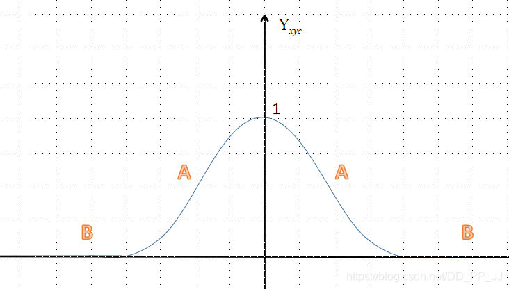
上图是一个简单的示意,纵坐标是{Y}_{xyc},分为A区(距离中心点较近,但是值在0-1之间)和B区(距离中心点很远接近于0)。
对于A区来说,由于其周围是一个高斯核生成的中心,Y_{xyc}的值是从1慢慢变到0。
举个例子(CenterNet中默认\alpha=2,\beta=4):
Y_{xyc}=0.8的情况下,
- 如果\hat{Y}_{xyc}=0.99,那么loss=(1-0.8)^4(0.99)^2log(1-0.99),这就是一个很大的loss值。
- 如果\hat{Y}_{xyc}=0.8, 那么loss=(1-0.8)^4(0.8)^2log(1-0.8), 这个loss就比较小。
-
如果\hat{Y}_{xyc}=0.5, 那么loss=(1-0.8)^4(0.5)^2log(1-0.5),
-
如果\hat{Y}_{xyc}=0.99,那么loss=(1-0.5)^4(0.99)^2log(1-0.99),这就是一个很大的loss值。
- 如果\hat{Y}_{xyc}=0.8, 那么loss=(1-0.5)^4(0.8)^2log(1-0.8), 这个loss就比较小。
- 如果\hat{Y}_{xyc}=0.5, 那么loss=(1-0.5)^4(0.5)^2log(1-0.5),
总结一下:为了防止预测值\hat{Y}_{xyc}过高接近于1,所以用(\hat{Y}_{xyc})^\alpha来惩罚Loss。而(1-Y_{xyc})^\beta这个参数距离中心越近,其值越小,这个权重是用来减轻惩罚力度。
对于B区来说,\hat{Y}_{xyc}的预测值理应是0,如果该值比较大比如为1,那么(\hat{Y}_{xyc})^\alpha作为权重会变大,惩罚力度也加大了。如果预测值接近于0,那么(\hat{Y}_{xyc})^\alpha会很小,让其损失比重减小。对于(1-Y_{xyc})^\beta来说,B区的值比较大,弱化了中心点周围其他负样本的损失比重。
2.2 offset loss
由于三个骨干网络输出的feature map的空间分辨率变为原来输入图像的四分之一。相当于输出feature map上一个像素点对应原始图像的4x4的区域,这会带来较大的误差,因此引入了偏置值和偏置的损失值。设骨干网络输出的偏置值为\hat{O}\in R^{\frac{W}{R}\times \frac{H}{R}\times 2}, 这个偏置值用L1 loss来训练:
p代表目标框中心点,R代表下采样倍数4,\tilde{p}=\lfloor \frac{p}{R} \rfloor, \frac{p}{R}-\tilde{p}代表偏差值。
2.3 size loss/wh loss
假设第k个目标,类别为c_k的目标框的表示为(x_1^{(k)},y_1^{(k)},x_2^{(k)},y_2^{(k)}),那么其中心点坐标位置为(\frac{x_1^{(k)}+x_2^{(k)}}{2}, \frac{y_1^{(k)}+y_2^{(k)}}{2}), 目标的长和宽大小为s_k=(x_2^{(k)}-x_1^{(k)},y_2^{(k)}-y_1^{(k)})。对长和宽进行训练的是L1 Loss函数:
其中\hat{S}\in R^{\frac{W}{R}\times \frac{H}{R}\times 2}是网络输出的结果。
2.4 CenterNet Loss
整体的损失函数是以上三者的综合,并且分配了不同的权重。 $$ L_{det}=L_k+\lambda_{size}L_{size}+\lambda_{offset}L_{offset} $$ 其中\lambda_{size}=0.1, \lambda_{offsize}=1
3. 代码解析
来自train.py中第173行开始进行loss计算:
# 得到heat map, reg, wh 三个变量
hmap, regs, w_h_ = zip(*outputs)

regs = [
_tranpose_and_gather_feature(r, batch['inds']) for r in regs
]
w_h_ = [
_tranpose_and_gather_feature(r, batch['inds']) for r in w_h_
]

# 分别计算loss
hmap_loss = _neg_loss(hmap, batch['hmap'])
reg_loss = _reg_loss(regs, batch['regs'], batch['ind_masks'])
w_h_loss = _reg_loss(w_h_, batch['w_h_'], batch['ind_masks'])

# 进行loss加权,得到最终loss
loss = hmap_loss + 1 * reg_loss + 0.1 * w_h_loss
上述transpose_and_gather_feature函数具体实现如下,主要功能是将ground truth中计算得到的对应中心点的值获取。
def _tranpose_and_gather_feature(feat, ind):
  # ind代表的是ground truth中设置的存在目标点的下角标
  feat = feat.permute(0, 2, 3, 1).contiguous()# from [bs c h w] to [bs, h, w, c]
  feat = feat.view(feat.size(0), -1, feat.size(3)) # to [bs, wxh, c]
  feat = _gather_feature(feat, ind)
  return feat

def _gather_feature(feat, ind, mask=None):
  # feat : [bs, wxh, c]
  dim = feat.size(2)
  # ind : [bs, index, c]
  ind = ind.unsqueeze(2).expand(ind.size(0), ind.size(1), dim)
  feat = feat.gather(1, ind) # 按照dim=1获取ind
  if mask is not None:
    mask = mask.unsqueeze(2).expand_as(feat)
    feat = feat[mask]
    feat = feat.view(-1, dim)
  return feat
3.1 hmap loss代码
调用:hmap_loss = _neg_loss(hmap, batch['hmap'])
def _neg_loss(preds, targets):
    ''' Modified focal loss. Exactly the same as CornerNet.
        Runs faster and costs a little bit more memory
        Arguments:
        preds (B x c x h x w)
        gt_regr (B x c x h x w)
    '''
    pos_inds = targets.eq(1).float()# heatmap为1的部分是正样本
    neg_inds = targets.lt(1).float()# 其他部分为负样本

    neg_weights = torch.pow(1 - targets, 4)# 对应(1-Yxyc)^4

    loss = 0
    for pred in preds: # 预测值
        # 约束在0-1之间
        pred = torch.clamp(torch.sigmoid(pred), min=1e-4, max=1 - 1e-4)
        pos_loss = torch.log(pred) * torch.pow(1 - pred, 2) * pos_inds
        neg_loss = torch.log(1 - pred) * torch.pow(pred,
                                                   2) * neg_weights * neg_inds
        num_pos = pos_inds.float().sum()
        pos_loss = pos_loss.sum()
        neg_loss = neg_loss.sum()

        if num_pos == 0:
            loss = loss - neg_loss # 只有负样本
        else:
            loss = loss - (pos_loss + neg_loss) / num_pos
    return loss / len(preds)
代码和以上公式一一对应,pos代表正样本,neg代表负样本。
3.2 reg & wh loss代码
调用:reg_loss = _reg_loss(regs, batch['regs'], batch['ind_masks'])
调用:w_h_loss = _reg_loss(w_h_, batch['w_h_'], batch['ind_masks'])
def _reg_loss(regs, gt_regs, mask):
    mask = mask[:, :, None].expand_as(gt_regs).float()
    loss = sum(F.l1_loss(r * mask, gt_regs * mask, reduction='sum') /
               (mask.sum() + 1e-4) for r in regs)
    return loss / len(regs)
4. 参考
[1]https://zhuanlan.zhihu.com/p/66048276
[2]http://xxx.itp.ac.cn/pdf/1904.07850
六、测试推理过程
这是CenterNet系列的最后一篇。本章主要讲CenterNet在推理过程中的数据加载和后处理部分代码。最后提供了一个已经配置好的数据集供大家使用。
代码注释在:https://github.com/pprp/SimpleCVReproduction/tree/master/CenterNet
1. eval部分数据加载
由于CenterNet是生成了一个heatmap进行的目标检测,而不是传统的基于anchor的方法,所以训练时候的数据加载和测试时的数据加载结果是不同的。并且在测试的过程中使用到了Test Time Augmentation(TTA),使用到了多尺度测试,翻转等。
在CenterNet中由于不需要非极大抑制,速度比较快。但是CenterNet如果在测试的过程中加入了多尺度测试,那就会调用soft nms将不同尺度的返回的框进行抑制。
class PascalVOC_eval(PascalVOC):
    def __init__(self, data_dir, split, test_scales=(1,), test_flip=False, fix_size=True, **kwargs):
        super(PascalVOC_eval, self).__init__(data_dir, split, **kwargs)
        # test_scale = [0.5,0.75,1,1.25,1.5]
        self.test_flip = test_flip
        self.test_scales = test_scales
        self.fix_size = fix_size

    def __getitem__(self, index):
        img_id = self.images[index]
        img_path = os.path.join(
            self.img_dir, self.coco.loadImgs(ids=[img_id])[0]['file_name'])
        image = cv2.imread(img_path)
        height, width = image.shape[0:2]

        out = {}
        for scale in self.test_scales:
            # 得到多个尺度的图片大小
            new_height = int(height * scale)
            new_width = int(width * scale)

            if self.fix_size:
                # fix size代表根据参数固定图片大小
                img_height, img_width = self.img_size['h'], self.img_size['w']
                center = np.array(
                    [new_width / 2., new_height / 2.], dtype=np.float32)
                scaled_size = max(height, width) * 1.0
                scaled_size = np.array(
                    [scaled_size, scaled_size], dtype=np.float32)
            else:
                # self.padding = 31  # 127 for hourglass
                img_height = (new_height | self.padding) + 1
                img_width = (new_width | self.padding) + 1
                # 按位或运算,找到最接近的[32,64,128,256,512]
                center = np.array(
                    [new_width // 2, new_height // 2], dtype=np.float32)
                scaled_size = np.array(
                    [img_width, img_height], dtype=np.float32)

            img = cv2.resize(image, (new_width, new_height))
            trans_img = get_affine_transform(
                center, scaled_size, 0, [img_width, img_height])
            img = cv2.warpAffine(img, trans_img, (img_width, img_height))

            img = img.astype(np.float32) / 255.
            img -= self.mean
            img /= self.std
            # from [H, W, C] to [1, C, H, W]
            img = img.transpose(2, 0, 1)[None, :, :, :]

            if self.test_flip: # 横向翻转
                img = np.concatenate((img, img[:, :, :, ::-1].copy()), axis=0)

            out[scale] = {'image': img,
                          'center': center,
                          'scale': scaled_size,
                          'fmap_h': img_height // self.down_ratio, # feature map的大小
                          'fmap_w': img_width // self.down_ratio}

        return img_id, out
以上是eval过程的数据加载部分的代码,主要有两个需要关注的点:
- 如果是多尺度会根据test_scale的值返回不同尺度的结果,每个尺度都有img,center等信息。这部分代码可以和test.py代码的多尺度处理一块理解。
- 尺度处理部分,有一个padding参数
img_height = (new_height | self.padding) + 1
img_width = (new_width | self.padding) + 1
这部分代码作用就是通过按位或运算,找到最接近的2的倍数-1作为最终的尺度。
'''
>>> 10 | 31
31
>>> 20 | 31
31
>>> 510 | 31
511
>>> 256 | 31
287
>>> 510 | 127
511
>>> 1000 | 127
1023
'''
例如:输入512,多尺度开启:0.5,0.7,1.5,那最终的结果是
512 x 0.5 | 31 = 287
512 x 0.7 | 31 = 383
512 x 1.5 | 31 = 799
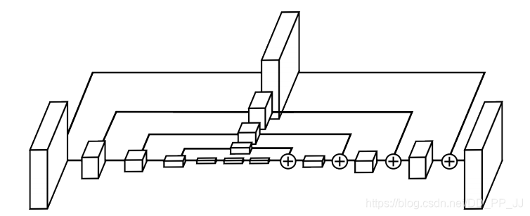
2. 推理过程

上图是CenterNet的结构图,使用的是PlotNeuralNet工具绘制。在推理阶段,输入图片通过骨干网络进行特征提取,然后对下采样得到的特征图进行预测,得到三个头,分别是offset head、wh head、heatmap head。
推理过程核心工作就是从heatmap提取得到需要的bounding box,具体的提取方法是使用了一个3x3的最大化池化,检查当前热点的值是否比周围8个临近点的值都大。然后取100个这样的点,再做筛选。
以上过程的核心函数是:
output = model(inputs[scale]['image'])[-1]
dets = ctdet_decode(*output, K=cfg.test_topk)
ctdet_decode这个函数功能就是将heatmap转化成bbox:
def ctdet_decode(hmap, regs, w_h_, K=100):
    '''
    hmap提取中心点位置为xs,ys
    regs保存的是偏置,需要加在xs,ys上,代表精确的中心位置
    w_h_保存的是对应目标的宽和高
    '''
    # dets = ctdet_decode(*output, K=cfg.test_topk)
    batch, cat, height, width = hmap.shape
    hmap = torch.sigmoid(hmap) # 归一化到0-1

    # if flip test
    if batch > 1: # batch > 1代表使用了翻转
        # img = np.concatenate((img, img[:, :, :, ::-1].copy()), axis=0)
        hmap = (hmap[0:1] + flip_tensor(hmap[1:2])) / 2
        w_h_ = (w_h_[0:1] + flip_tensor(w_h_[1:2])) / 2
        regs = regs[0:1]
    batch = 1
    # 这里的nms和带anchor的目标检测方法中的不一样,这里使用的是3x3的maxpool筛选
    hmap = _nms(hmap)  # perform nms on heatmaps
    # 找到前K个极大值点代表存在目标
    scores, inds, clses, ys, xs = _topk(hmap, K=K)

    regs = _tranpose_and_gather_feature(regs, inds)

    regs = regs.view(batch, K, 2)

    xs = xs.view(batch, K, 1) + regs[:, :, 0:1]
    ys = ys.view(batch, K, 1) + regs[:, :, 1:2]

    w_h_ = _tranpose_and_gather_feature(w_h_, inds)
    w_h_ = w_h_.view(batch, K, 2)

    clses = clses.view(batch, K, 1).float()
    scores = scores.view(batch, K, 1)

    # xs,ys是中心坐标,w_h_[...,0:1]是w,1:2是h
    bboxes = torch.cat([xs - w_h_[..., 0:1] / 2,
                        ys - w_h_[..., 1:2] / 2,
                        xs + w_h_[..., 0:1] / 2,
                        ys + w_h_[..., 1:2] / 2], dim=2)
    detections = torch.cat([bboxes, scores, clses], dim=2)
    return detections
第一步
将hmap归一化,使用了sigmoid函数
hmap = torch.sigmoid(hmap) # 归一化到0-1
第二步
进入_nms函数:
def _nms(heat, kernel=3):
    hmax = F.max_pool2d(heat, kernel, stride=1, padding=(kernel - 1) // 2)
    keep = (hmax == heat).float() # 找到极大值点
    return heat * keep
hmax代表特征图经过3x3卷积以后的结果,keep为极大点的位置,返回的结果是筛选后的极大值点,其余不符合8-近邻极大值点的都归为0。
这时候通过heatmap得到了满足8近邻极大值点的所有值。
这里的nms曾经在群里讨论过,有群友认为仅通过3x3的并不合理,可以尝试使用3x3,5x5,7x7这样的maxpooling,相当于也进行了多尺度测试。据群友说能提高一点点mAP。
第三步
进入_topk函数,这里K是一个超参数,CenterNet中设置K=100
def _topk(scores, K=40):
    # score shape : [batch, class , h, w]
    batch, cat, height, width = scores.size()

    # to shape: [batch , class, h * w] 分类别,每个class channel统计最大值
    # topk_scores和topk_inds分别是前K个score和对应的id
    topk_scores, topk_inds = torch.topk(scores.view(batch, cat, -1), K)

    topk_inds = topk_inds % (height * width)
    # 找到横纵坐标
    topk_ys = (topk_inds / width).int().float()
    topk_xs = (topk_inds % width).int().float()

    # to shape: [batch , class * h * w] 这样的结果是不分类别的,全体class中最大的100个
    topk_score, topk_ind = torch.topk(topk_scores.view(batch, -1), K)

    # 所有类别中找到最大值
    topk_clses = (topk_ind / K).int()

    topk_inds = _gather_feature(topk_inds.view(
        batch, -1, 1), topk_ind).view(batch, K)

    topk_ys = _gather_feature(topk_ys.view(
        batch, -1, 1), topk_ind).view(batch, K)

    topk_xs = _gather_feature(topk_xs.view(
        batch, -1, 1), topk_ind).view(batch, K)

    return topk_score, topk_inds, topk_clses, topk_ys, topk_xs
torch.topk的一个demo如下:
>>> x
array([[0.11530714, 0.014376  , 0.23392263, 0.48629663],
       [0.59611302, 0.83697236, 0.27330404, 0.17728915],
       [0.36443852, 0.46562404, 0.73033529, 0.44751189]])
>>> torch.topk(torch.from_numpy(x), 3)
torch.return_types.topk(
    values=tensor([[0.4863, 0.2339, 0.1153],
                   [0.8370, 0.5961, 0.2733],
                   [0.7303, 0.4656, 0.4475]], dtype=torch.float64),
    indices=tensor([[3, 2, 0],
                    [1, 0, 2],
                    [2, 1, 3]]))
topk_scores和topk_inds分别是前K个score和对应的id。
-
topk_scores 形状【batch, class, K】K代表得分最高的前100个点, 其保存的内容是每个类别前100个最大的score。
-
topk_inds 形状 【batch, class, K】class代表80个类别channel,其保存的是每个类别对应100个score的下角标。
- topk_score 形状 【batch, K】,通过gather feature 方法获取,其保存的是全部类别前100个最大的score。
- topk_ind 形状 【batch , K】,代表通过topk调用结果的下角标, 其保存的是全部类别对应的100个score的下角标。
- topk_inds、topk_ys、topk_xs三个变量都经过gather feature函数,其主要功能是从对应张量中根据下角标提取结果,具体函数如下:
def _gather_feature(feat, ind, mask=None):
  dim = feat.size(2)
  ind = ind.unsqueeze(2).expand(ind.size(0), ind.size(1), dim)
  feat = feat.gather(1, ind) # 按照dim=1获取ind
  if mask is not None:
    mask = mask.unsqueeze(2).expand_as(feat)
    feat = feat[mask]
    feat = feat.view(-1, dim)
  return feat
以topk_inds为例(K=100,class=80)
feat (topk_inds) 形状为:【batch, 80x100, 1】
ind (topk_ind) 形状为:【batch,100】
ind = ind.unsqueeze(2).expand(ind.size(0), ind.size(1), dim)扩展一个位置,ind形状变为:【batch, 100, 1】
feat = feat.gather(1, ind)按照dim=1获取ind,为了方便理解和回忆,这里举一个例子:
>>> import torch
>>> a = torch.randn(1, 10)
>>> b = torch.tensor([[3,4,5]])
>>> a.gather(1, b)
tensor([[ 0.7257, -0.4977,  1.2522]])
>>> a
tensor([[ 1.0684, -0.9655,  0.7381,  0.7257, -0.4977,  1.2522,  1.5084,  0.2669,
         -0.5471,  0.5998]])
相当于是feat根据ind的角标的值获取到了对应feat位置上的结果。最终feat形状为【batch,100,1】
第四步
经过topk函数,得到了四个返回值,topk_score、topk_inds、topk_ys、topk_xs四个参数的形状都是【batch, 100】,其中topk_inds是每张图片的前100个最大的值对应的index。
regs = _tranpose_and_gather_feature(regs, inds)
w_h_ = _tranpose_and_gather_feature(w_h_, inds)
transpose_and_gather_feat函数功能是将topk得到的index取值,得到对应前100的regs和wh的值。
def _tranpose_and_gather_feature(feat, ind):
  # ind代表的是ground truth中设置的存在目标点的下角标
  feat = feat.permute(0, 2, 3, 1).contiguous()# from [bs c h w] to [bs, h, w, c]
  feat = feat.view(feat.size(0), -1, feat.size(3)) # to [bs, wxh, c]
  feat = _gather_feature(feat, ind) # 从中取得ind对应值
  return feat
到这一步为止,可以将top100的score、wh、regs等值提取,并且得到对应的bbox,最终ctdet_decode返回了detections变量。
3. 数据集
之前在CenterNet系列第一篇PyTorch版CenterNet训练自己的数据集中讲解了如何配置数据集,为了更方便学习和调试这部分代码,笔者从github上找到了行云大佬之前分享过的浣熊数据集,这个数据集仅有200张图片,方便大家快速训练和debug。
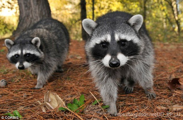
链接:https://pan.baidu.com/s/1unK-QZKDDaGwCrHrOFCXEA 提取码:pdcv
以上数据集已经制作好了,只要按照第一篇文章中将DCN、NMS等编译好,就可以直接使用。
5. 参考
[1]https://blog.csdn.net/fsalicealex/article/details/91955759
[2]https://zhuanlan.zhihu.com/p/66048276
[3]https://zhuanlan.zhihu.com/p/85194783
七、总结
在这里将所有的资源重新罗列一下:
- 数据集
链接:https://pan.baidu.com/s/1unK-QZKDDaGwCrHrOFCXEA 提取码:pdcv
- 代码
注释:https://github.com/pprp/SimpleCVReproduction/tree/master/CenterNet
原版:https://github.com/zzzxxxttt/pytorch_simple_CenterNet_45
- 博客
https://www.jianshu.com/p/7dc88493a31f
https://zhuanlan.zhihu.com/p/96856635
https://zhuanlan.zhihu.com/p/76378871
https://www.cnblogs.com/shine-lee/p/9671253.html
https://zhuanlan.zhihu.com/p/66048276
https://zhuanlan.zhihu.com/p/85194783
https://medium.com/visionwizard/centernet-objects-as-points-a-comprehensive-guide-2ed9993c48bc
本电子书是将首发于GiantPandaCV公众号的CenterNet的一个系列的文章组合而成的。由于笔者水平有限,以上内容可能会存在一些疏漏和不足,如果有批评指正,欢迎添加笔者微信

本文总阅读量次