一、 YOLO cfg文件解析
与其他框架不同,Darknet构建网络架构不是通过代码直接堆叠,而是通过解析cfg文件进行生成的。cfg文件格式是有一定规则,虽然比较简单,但是有些地方需要对yolov3有一定程度的熟悉,才能正确设置。
下边以yolov3.cfg为例进行讲解。
1. Net层
[net]
#Testing
#batch=1
#subdivisions=1
#在测试的时候,设置batch=1,subdivisions=1
#Training
batch=16
subdivisions=4
#这里的batch与普遍意义上的batch不是一致的。
#训练的过程中将一次性加载16张图片进内存,然后分4次完成前向传播,每次4张。
#经过16张图片的前向传播以后,进行一次反向传播。
width=416
height=416
channels=3
#设置图片进入网络的宽、高和通道个数。
#由于YOLOv3的下采样一般是32倍,所以宽高必须能被32整除。
#多尺度训练选择为32的倍数最小320*320,最大608*608。
#长和宽越大,对小目标越好,但是占用显存也会高,需要权衡。
momentum=0.9
#动量参数影响着梯度下降到最优值得速度。
decay=0.0005
#权重衰减正则项,防止过拟合。
angle=0
#数据增强,设置旋转角度。
saturation = 1.5
#饱和度
exposure = 1.5
#曝光量
hue=.1
#色调

learning_rate=0.001
#学习率:刚开始训练时可以将学习率设置的高一点,而一定轮数之后,将其减小。
#在训练过程中,一般根据训练轮数设置动态变化的学习率。
burn_in=1000
max_batches = 500200
#最大batch
policy=steps
#学习率调整的策略,有以下policy:
#constant, steps, exp, poly, step, sig, RANDOM,constant等方式
#调整学习率的policy,
#有如下policy:constant, steps, exp, poly, step, sig, RANDOM。
#steps#比较好理解,按照steps来改变学习率。

steps=400000,450000
scales=.1,.1
#在达到40000、45000的时候将学习率乘以对应的scale
2. 卷积层
[convolutional]
batch_normalize=1
#是否做BN操作
filters=32
#输出特征图的数量
size=3
#卷积核的尺寸
stride=1
#做卷积运算的步长
pad=1
#如果pad为0,padding由padding参数指定。
#如果pad为1,padding大小为size/2,padding应该是对输入图像左边缘拓展的像素数量
activation=leaky
#激活函数的类型:logistic,loggy,relu,
#elu,relie,plse,hardtan,lhtan,
#linear,ramp,leaky,tanh,stair
# alexeyAB版添加了mish, swish, nrom_chan等新的激活函数
feature map计算公式:
3. 下采样
可以通过调整卷积层参数进行下采样:
[convolutional]
batch_normalize=1
filters=128
size=3
stride=2
pad=1
activation=leaky
可以通过带入以上公式,可以得到OutFeature是InFeature的一半。
也可以使用maxpooling进行下采样:
[maxpool]
size=2
stride=2
4. 上采样
[upsample]
stride=2
上采样是通过线性插值实现的。
5. Shortcut和Route层
[shortcut]
from=-3
activation=linear
#shortcut操作是类似ResNet的跨层连接,参数from是−3,
#意思是shortcut的输出是当前层与先前的倒数第三层相加而得到。
# 通俗来讲就是add操作

[route]
layers = -1, 36
# 当属性有两个值,就是将上一层和第36层进行concate
#即沿深度的维度连接,这也要求feature map大小是一致的。
[route]
layers = -4
#当属性只有一个值时,它会输出由该值索引的网络层的特征图。
#本例子中就是提取从当前倒数第四个层输出
6. YOLO层
[convolutional]
size=1
stride=1
pad=1
filters=18
#每一个[region/yolo]层前的最后一个卷积层中的
#filters=num(yolo层个数)*(classes+5) ,5的意义是5个坐标,
#代表论文中的tx,ty,tw,th,po
#这里类别个数为1,(1+5)*3=18
activation=linear

[yolo]
mask = 6,7,8
#训练框mask的值是0,1,2,
#这意味着使用第一,第二和第三个anchor
anchors = 10,13,  16,30,  33,23,  30,61,  62,45,\
          59,119,  116,90,  156,198,  373,326
# 总共有三个检测层,共计9个anchor
# 这里的anchor是由kmeans聚类算法得到的。
classes=1
#类别个数
num=9
#每个grid预测的BoundingBox num/yolo层个数
jitter=.3
#利用数据抖动产生更多数据,
#属于TTA(Test Time Augmentation)
ignore_thresh = .5
# ignore_thresh 指得是参与计算的IOU阈值大小。
#当预测的检测框与ground true的IOU大于ignore_thresh的时候,
#不会参与loss的计算,否则,检测框将会参与损失计算。
#目的是控制参与loss计算的检测框的规模,当ignore_thresh过于大,
#接近于1的时候,那么参与检测框回归loss的个数就会比较少,同时也容易造成过拟合;
#而如果ignore_thresh设置的过于小,那么参与计算的会数量规模就会很大。
#同时也容易在进行检测框回归的时候造成欠拟合。
#ignore_thresh 一般选取0.5-0.7之间的一个值
# 小尺度(13*13)用的是0.7,
# 大尺度(26*26)用的是0.5。
7. 模块总结
Darket-53结构如下图所示:
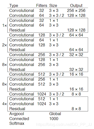
它是由重复的类似于ResNet的模块组成的,其下采样是通过卷积来完成的。通过对cfg文件的观察,提出了以下总结:
不改变feature大小的模块:
- 残差模块:
[convolutional]
batch_normalize=1
filters=128
size=1
stride=1
pad=1
activation=leaky

[convolutional]
batch_normalize=1
filters=256
size=3
stride=1
pad=1
activation=leaky

[shortcut]
from=-3
activation=linear
- 1×1卷积:可以降低计算量
[convolutional]
batch_normalize=1
filters=512
size=1
stride=1
pad=1
activation=leaky
- 普通3×3卷积:可以对filter个数进行调整
[convolutional]
batch_normalize=1
filters=1024
size=3
stride=1
pad=1
activation=leaky
改变feature map大小
- feature map减半:
[maxpool]
size=2
stride=2
或者
[convolutional]
batch_normalize=1
filters=128
size=3
stride=2
pad=1
activation=leaky
- feature map加倍:
[maxpool]
size=2
stride=1
特征融合操作
- 使用Route层获取指定的层(13×13)。
- 添加卷积层进行学习但不改变feature map大小。
- 进行上采样(26×26)。
- 从backbone中找到对应feature map大小的层进行Route或者Shortcut(26×26)。
- 融合完成。
后记:以上就是笔者之前使用darknet过程中收集和总结的一些经验,掌握以上内容并读懂yolov3论文后,就可以着手运行代码了。目前使用与darknet一致的cfg文件解析的有一些,比如原版Darknet,AlexeyAB版本的Darknet,还有一个pytorch版本的yolov3。AlexeyAB版本的添加了很多新特性,比如 [conv_lstm], [scale_channels] SE/ASFF/BiFPN, [local_avgpool], [sam], [Gaussian_yolo], [reorg3d] (fixed [reorg]), fixed [batchnorm]等等。而pytorch版本的yolov3可以很方便的添加我们需要的功能。之后将会对这个版本进行改进,添加孔洞卷积、SE、CBAM、SK等模块。
二、代码配置和数据集处理
前言:本文是讲的是如何配置pytorch版本的yolov3、数据集处理、常用的命令等内容。该库的数据集格式既不是VOC2007格式也不是MS COCO的格式,而是一种新的格式,跟着文章一步一步来,很简单。另外我们公众号针对VOC2007格式数据集转化为本库所需要格式特意开发了一个简单的数据处理库。
1. 环境搭建
- 将github库download下来。
git clone https://github.com/ultralytics/yolov3.git
- 建议在linux环境下使用anaconda进行搭建
conda create -n yolov3 python=3.7
- 安装需要的软件
pip install -r requirements.txt
环境要求:
- python >= 3.7
- pytorch >= 1.1
- numpy
- tqdm
- opencv-python
其中只需要注意pytorch的安装:
到https://pytorch.org/中根据操作系统,python版本,cuda版本等选择命令即可。
2. 数据集构建
2.1 xml文件生成需要Labelimg软件
在Windows下使用LabelImg软件进行标注:
- 使用快捷键:
Ctrl + u  加载目录中的所有图像,鼠标点击Open dir同功能
Ctrl + r  更改默认注释目标目录(xml文件保存的地址)
Ctrl + s  保存
Ctrl + d  复制当前标签和矩形框
space     将当前图像标记为已验证
w         创建一个矩形框
d         下一张图片
a         上一张图片
del       删除选定的矩形框
Ctrl++    放大
Ctrl--    缩小
↑→↓←        键盘箭头移动选定的矩形框
2.2 VOC2007 数据集格式
-data
    - VOCdevkit2007
        - VOC2007
            - Annotations (标签XML文件,用对应的图片处理工具人工生成的)
            - ImageSets (生成的方法是用sh或者MATLAB语言生成)
                - Main
                    - test.txt
                    - train.txt
                    - trainval.txt
                    - val.txt
            - JPEGImages(原始文件)
            - labels (xml文件对应的txt文件)
通过以上软件主要构造好JPEGImages和Annotations文件夹中内容,Main文件夹中的txt文件可以通过以下python脚本生成:
import os
import random

trainval_percent = 0.9
train_percent = 1
xmlfilepath = 'Annotations'
txtsavepath = 'ImageSets\Main'
total_xml = os.listdir(xmlfilepath)

num=len(total_xml)
list=range(num)
tv=int(num*trainval_percent)
tr=int(tv*train_percent)
trainval= random.sample(list,tv)
train=random.sample(trainval,tr)

ftrainval = open('ImageSets/Main/trainval.txt', 'w')
ftest = open('ImageSets/Main/test.txt', 'w')
ftrain = open('ImageSets/Main/train.txt', 'w')
fval = open('ImageSets/Main/val.txt', 'w')

for i  in list:
    name=total_xml[i][:-4]+'\n'
    if i in trainval:
        ftrainval.write(name)
        if i in train:
            ftrain.write(name)
        else:
            fval.write(name)
    else:
        ftest.write(name)

ftrainval.close()
ftrain.close()
fval.close()
ftest.close()
接下来生成labels文件夹中的txt文件,voc_label.py文件具体内容如下:
# -*- coding: utf-8 -*-
"""
Created on Tue Oct  2 11:42:13 2018
将本文件放到VOC2007目录下,然后就可以直接运行
需要修改的地方:
1. sets中替换为自己的数据集
2. classes中替换为自己的类别
3. 将本文件放到VOC2007目录下
4. 直接开始运行
"""

import xml.etree.ElementTree as ET
import pickle
import os
from os import listdir, getcwd
from os.path import join
sets=[('2007', 'train'), ('2007', 'val'), ('2007', 'test')]  #替换为自己的数据集
classes = ["person"]     #修改为自己的类别

#进行归一化
def convert(size, box):
    dw = 1./(size[0])
    dh = 1./(size[1])
    x = (box[0] + box[1])/2.0 - 1
    y = (box[2] + box[3])/2.0 - 1
    w = box[1] - box[0]
    h = box[3] - box[2]
    x = x*dw
    w = w*dw
    y = y*dh
    h = h*dh
    return (x,y,w,h)

def convert_annotation(year, image_id):
    in_file = open('VOC%s/Annotations/%s.xml'%(year, image_id))  #将数据集放于当前目录下
    out_file = open('VOC%s/labels/%s.txt'%(year, image_id), 'w')
    tree=ET.parse(in_file)
    root = tree.getroot()
    size = root.find('size')
    w = int(size.find('width').text)
    h = int(size.find('height').text)
    for obj in root.iter('object'):
        difficult = obj.find('difficult').text
        cls = obj.find('name').text
        if cls not in classes or int(difficult)==1:
            continue
        cls_id = classes.index(cls)
        xmlbox = obj.find('bndbox')
        b = (float(xmlbox.find('xmin').text), float(xmlbox.find('xmax').text), float(xmlbox.find('ymin').text), float(xmlbox.find('ymax').text))
        bb = convert((w,h), b)
        out_file.write(str(cls_id) + " " + " ".join([str(a) for a in bb]) + '\n')
wd = getcwd()
for year, image_set in sets:
    if not os.path.exists('VOC%s/labels/'%(year)):
        os.makedirs('VOC%s/labels/'%(year))
    image_ids = open('VOC%s/ImageSets/Main/%s.txt'%(year, image_set)).read().strip().split()
    list_file = open('%s_%s.txt'%(year, image_set), 'w')
    for image_id in image_ids:
        list_file.write('VOC%s/JPEGImages/%s.jpg\n'%(year, image_id))
        convert_annotation(year, image_id)
    list_file.close()
到底为止,VOC格式数据集构造完毕,但是还需要继续构造符合darknet格式的数据集(coco)。
需要说明的是:如果打算使用coco评价标准,需要构造coco中json格式,如果要求不高,只需要VOC格式即可,使用作者写的mAP计算程序即可。
2.3 创建*.names file,
其中保存的是你的所有的类别,每行一个类别,如data/coco.names:
person
2.4 更新data/coco.data,其中保存的是很多配置信息
classes = 1 # 改成你的数据集的类别个数
train = ./data/2007_train.txt # 通过voc_label.py文件生成的txt文件
valid = ./data/2007_test.txt # 通过voc_label.py文件生成的txt文件
names = data/coco.names # 记录类别
backup = backup/ # 在本库中没有用到
eval = coco # 选择map计算方式
2.5 更新cfg文件,修改类别相关信息
打开cfg文件夹下的yolov3.cfg文件,大体而言,cfg文件记录的是整个网络的结构,是核心部分,具体内容讲解请参考之前的文章:【从零开始学习YOLOv3】1. YOLOv3的cfg文件解析与总结
只需要更改每个[yolo]层前边卷积层的filter个数即可:
每一个[region/yolo]层前的最后一个卷积层中的 filters=预测框的个数(mask对应的个数,比如mask=0,1,2, 代表使用了anchors中的前三对,这里预测框个数就应该是3*(classes+5) ,5的意义是5个坐标(论文中的tx,ty,tw,th,po),3的意义就是用了3个anchor。
举个例子:假如我有三个类,n = 3, 那么filter = 3 × (n+5) = 24
[convolutional]
size=1
stride=1
pad=1
filters=255 # 改为 24
activation=linear


[yolo]
mask = 6,7,8
anchors = 10,13,  16,30,  33,23,  30,61,  62,45,  59,119,  116,90,  156,198,  373,326
classes=80 # 改为 3
num=9
jitter=.3
ignore_thresh = .7
truth_thresh = 1
random=1
2.6 数据集格式说明
- yolov3
    - data
      - 2007_train.txt
      - 2007_test.txt
      - coco.names
      - coco.data
      - annotations(json files)
      - images(将2007_train.txt中的图片放到train2014文件夹中,test同理)
        - train2014
          - 0001.jpg
          - 0002.jpg
        - val2014
          - 0003.jpg
          - 0004.jpg
      - labels(voc_labels.py生成的内容需要重新组织一下)
        - train2014
          - 0001.txt
          - 0002.txt
        - val2014
          - 0003.txt
          - 0004.txt
      - samples(存放待测试图片)
2007_train.txt内容示例:
/home/dpj/yolov3-master/data/images/val2014/Cow_1192.jpg
/home/dpj/yolov3-master/data/images/val2014/Cow_1196.jpg
.....
注意images和labels文件架构一致性,因为txt是通过简单的替换得到的:
images -> labels
.jpg -> .txt
具体内容可以在datasets.py文件中找到详细的替换。
3. 训练模型
预训练模型:
- Darknet
*.weightsformat:https://pjreddie.com/media/files/yolov3.weights - PyTorch
*.ptformat:https://drive.google.com/drive/folders/1uxgUBemJVw9wZsdpboYbzUN4bcRhsuAI
开始训练:
python train.py --data data/coco.data --cfg cfg/yolov3.cfg
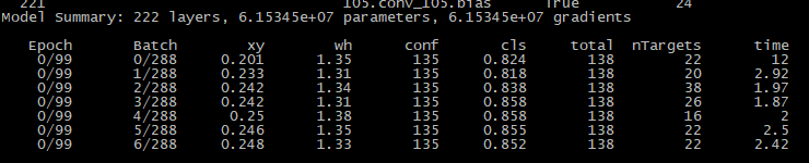
如果日志正常输出那证明可以运行了
如果中断了,可以恢复训练
python train.py --data data/coco.data --cfg cfg/yolov3.cfg --resume
4. 测试模型
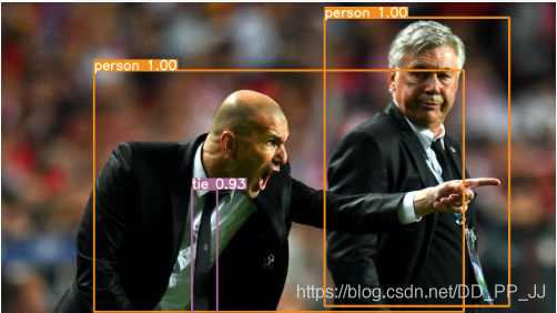
将待测试图片放到data/samples中,然后运行
python detect.py --cfg cfg/yolov3.cfg --weights weights/best.pt
目前该文件中也可以放入视频进行视频目标检测。
- Image:
--source file.jpg - Video:
--source file.mp4 - Directory:
--source dir/ - Webcam:
--source 0 - RTSP stream:
--source rtsp://170.93.143.139/rtplive/470011e600ef003a004ee33696235daa - HTTP stream:
--source http://wmccpinetop.axiscam.net/mjpg/video.mjpg
5. 评估模型
python test.py --weights weights/best.pt
如果使用cocoAPI使用以下命令:
$ python3 test.py --img-size 608 --iou-thr 0.6 --weights ultralytics68.pt --cfg yolov3-spp.cfg

Namespace(batch_size=32, cfg='yolov3-spp.cfg', conf_thres=0.001, data='data/coco2014.data', device='', img_size=608, iou_thres=0.6, save_json=True, task='test', weights='ultralytics68.pt')
Using CUDA device0 _CudaDeviceProperties(name='Tesla V100-SXM2-16GB', total_memory=16130MB)
               Class    Images   Targets         P         R   mAP@0.5        F1: 100% 157/157 [03:30<00:00,  1.16it/s]
                 all     5e+03  3.51e+04    0.0353     0.891     0.606    0.0673
 Average Precision  (AP) @[ IoU=0.50:0.95 | area=   all | maxDets=100 ] = 0.409
 Average Precision  (AP) @[ IoU=0.50      | area=   all | maxDets=100 ] = 0.615
 Average Precision  (AP) @[ IoU=0.75      | area=   all | maxDets=100 ] = 0.437
 Average Precision  (AP) @[ IoU=0.50:0.95 | area= small | maxDets=100 ] = 0.242
 Average Precision  (AP) @[ IoU=0.50:0.95 | area=medium | maxDets=100 ] = 0.448
 Average Precision  (AP) @[ IoU=0.50:0.95 | area= large | maxDets=100 ] = 0.519
 Average Recall     (AR) @[ IoU=0.50:0.95 | area=   all | maxDets=  1 ] = 0.337
 Average Recall     (AR) @[ IoU=0.50:0.95 | area=   all | maxDets= 10 ] = 0.557
 Average Recall     (AR) @[ IoU=0.50:0.95 | area=   all | maxDets=100 ] = 0.612
 Average Recall     (AR) @[ IoU=0.50:0.95 | area= small | maxDets=100 ] = 0.438
 Average Recall     (AR) @[ IoU=0.50:0.95 | area=medium | maxDets=100 ] = 0.658
 Average Recall     (AR) @[ IoU=0.50:0.95 | area= large | maxDets=100 ] = 0.746
mAP计算
- mAP@0.5 run at
--iou-thr 0.5, mAP@0.5...0.95 run at--iou-thr 0.7
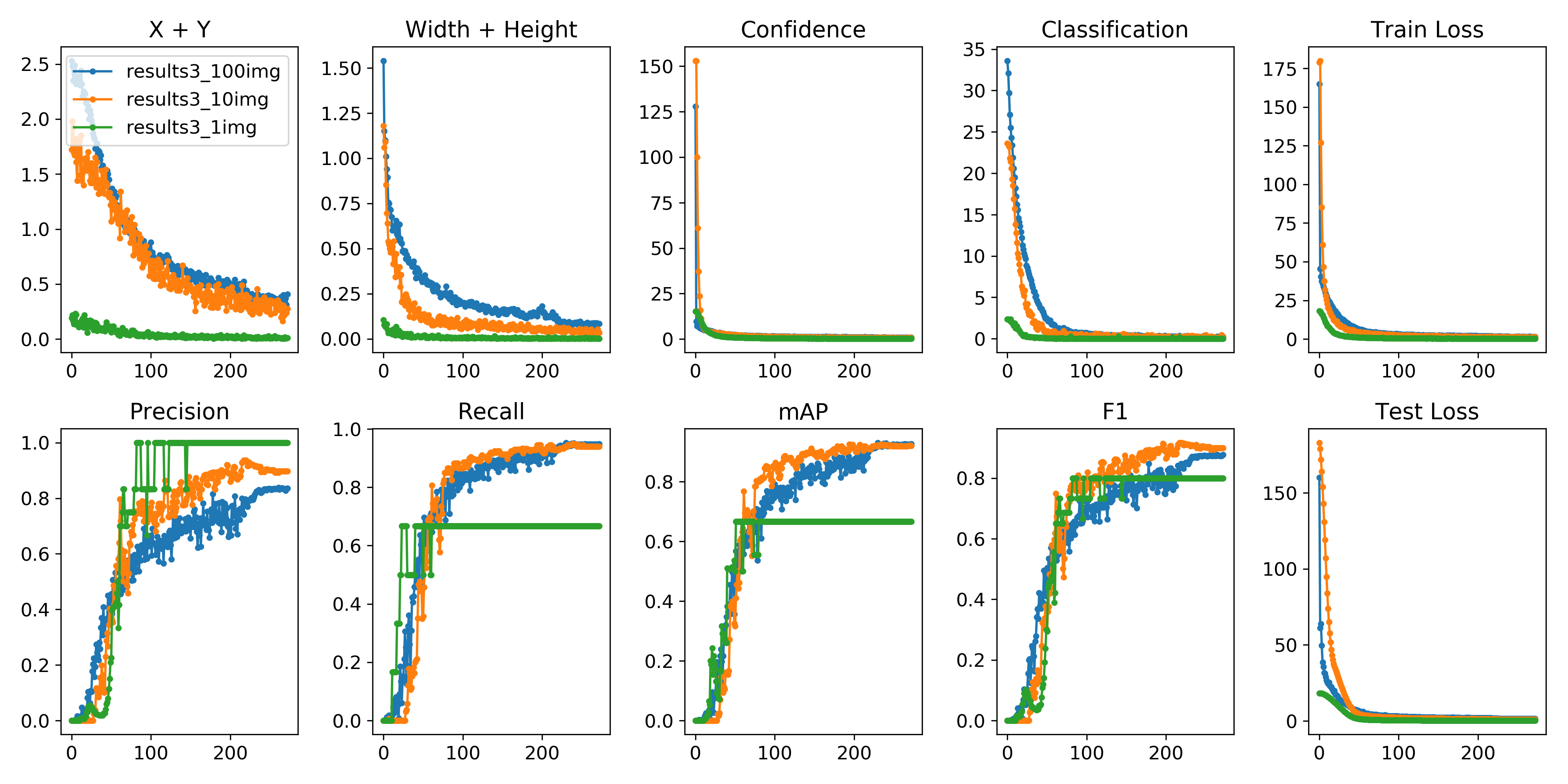
6. 可视化
可以使用python -c from utils import utils;utils.plot_results()
创建drawLog.py
def plot_results():
    # Plot YOLO training results file 'results.txt'
    import glob
    import numpy as np
    import matplotlib.pyplot as plt
    #import os; os.system('rm -rf results.txt && wget https://storage.googleapis.com/ultralytics/results_v1_0.txt')

    plt.figure(figsize=(16, 8))
    s = ['X', 'Y', 'Width', 'Height', 'Objectness', 'Classification', 'Total Loss', 'Precision', 'Recall', 'mAP']
    files = sorted(glob.glob('results.txt'))
    for f in files:
        results = np.loadtxt(f, usecols=[2, 3, 4, 5, 6, 7, 8, 17, 18, 16]).T  # column 16 is mAP
        n = results.shape[1]
        for i in range(10):
            plt.subplot(2, 5, i + 1)
            plt.plot(range(1, n), results[i, 1:], marker='.', label=f)
            plt.title(s[i])
            if i == 0:
                plt.legend()
    plt.savefig('./plot.png')
if __name__ == "__main__":
    plot_results()
7. 数据集配套代码
如果你看到这里了,恭喜你,你可以避开以上略显复杂的数据处理。我们提供了一套代码,集成了以上脚本,只需要你有jpg图片和对应的xml文件,就可以直接生成符合要求的数据集,然后按照要求修改一些代码即可。
代码地址:https://github.com/pprp/voc2007_for_yolo_torch
请按照readme中进行处理就可以得到数据集。
后记:这套代码一直由一个外国的团队进行维护,也添加了很多新的trick。目前已获得了3.3k个star,1k fork。不仅如此,其团队会经常回复issue,目前也有接近1k的issue。只要处理过一遍数据,就会了解到这个库的亮点,非常容易配置,不需要进行编译等操作,易用性极强。再加上提供的配套数据处理代码,在短短10多分钟就可以配置好。(✪ω✪)
这是这个系列第二篇内容,之后我们将对yolov3进行代码级别的学习,也会学习一下这个库提供的新的特性,比如说超参数进化,权重采样机制、loss计算、Giou处理等。希望各位多多关注。
参考内容:
官方代码:https://github.com/ultralytics/yolov3
官方讲解:https://github.com/ultralytics/yolov3/wiki/Train-Custom-Data
数据集配置库:https://github.com/pprp/voc2007_for_yolo_torch
三、YOLOv3的数据组织与处理
前言:本文主要讲YOLOv3中数据加载部分,主要解析的代码在utils/datasets.py文件中。通过对数据组织、加载、处理部分代码进行解读,能帮助我们更快地理解YOLOv3所要求的数据输出要求,也将有利于对之后训练部分代码进行理解。
1. 标注格式
在上一篇【从零开始学习YOLOv3】2. YOLOv3中的代码配置和数据集构建 中,使用到了voc_label.py,其作用是将xml文件转成txt文件格式,具体文件如下:
# class id, x, y, w, h
0 0.8604166666666666 0.5403899721448469 0.058333333333333334 0.055710306406685235
其中的x,y 的意义是归一化以后的框的中心坐标,w,h是归一化后的框的宽和高。
具体的归一化方式为:
def convert(size, box):
    '''
    size是图片的长和宽
    box是xmin,xmax,ymin,ymax坐标值
    '''
    dw = 1. / (size[0])
    dh = 1. / (size[1])
    # 得到长和宽的缩放比
    x = (box[0] + box[1])/2.0 - 1
    y = (box[2] + box[3])/2.0 - 1
    w = box[1] - box[0]
    h = box[3] - box[2]
    # 分别计算中心点坐标,框的宽和高
    x = x * dw
    w = w * dw
    y = y * dh
    h = h * dh
    # 按照图片长和宽进行归一化
    return (x,y,w,h)
可以看出,归一化都是相对于图片的宽和高进行归一化的。
2. 调用
下边是train.py文件中的有关数据的调用:
# Dataset
dataset = LoadImagesAndLabels(train_path, img_size, batch_size,
                              augment=True,
                              hyp=hyp,  # augmentation hyperparameters
                              rect=opt.rect,  # rectangular training
                              cache_labels=True,
                              cache_images=opt.cache_images)

batch_size = min(batch_size, len(dataset))

# 使用多少个线程加载数据集
nw = min([os.cpu_count(), batch_size if batch_size > 1 else 0, 1])

dataloader = DataLoader(dataset,
                        batch_size=batch_size,
                        num_workers=nw,
                        shuffle=not opt.rect,
                        # Shuffle=True
                        #unless rectangular training is used
                        pin_memory=True,
                        collate_fn=dataset.collate_fn)
在pytorch中,数据集加载主要是重构datasets类,然后再使用dataloader中加载dataset,就构建好了数据部分。
下面是一个简单的使用模板:
import os
from torch.utils.data import Dataset
from torch.utils.data import DataLoader

# 根据自己的数据集格式进行重构
class MyDataset(Dataset):
    def __init__(self):
        #下载数据、初始化数据,都可以在这里完成
        xy = np.loadtxt('label.txt', delimiter=',', dtype=np.float32)
        # 使用numpy读取数据
        self.x_data = torch.from_numpy(xy[:, 0:-1])
        self.y_data = torch.from_numpy(xy[:, [-1]])
        self.len = xy.shape[0]

    def __getitem__(self, index):
        # dataloader中使用该方法,通过index进行访问
        return self.x_data[index], self.y_data[index]

    def __len__(self):
        # 查询数据集中数量,可以通过len(mydataset)得到
        return self.len

# 实例化这个类,然后我们就得到了Dataset类型的数据,记下来就将这个类传给DataLoader,就可以了。
myDataset = MyDataset()

# 构建dataloader
train_loader = DataLoader(dataset=myDataset,
                          batch_size=32,
                          shuffle=True)

for epoch in range(2):
    for i, data in enumerate(train_loader2):
        # 将数据从 train_loader 中读出来,一次读取的样本数是32个
        inputs, labels = data
        # 将这些数据转换成Variable类型
        inputs, labels = Variable(inputs), Variable(labels)
        # 模型训练...
通过以上模板就能大致了解pytorch中的数据加载机制,下面开始介绍YOLOv3中的数据加载。
3. YOLOv3中的数据加载
下面解析的是LoadImagesAndLabels类中的几个主要的函数:
3.1 init函数
init函数中包含了大部分需要处理的数据
class LoadImagesAndLabels(Dataset):  # for training/testing
    def __init__(self,
                 path,
                 img_size=416,
                 batch_size=16,
                 augment=False,
                 hyp=None,
                 rect=False,
                 image_weights=False,
                 cache_labels=False,
                 cache_images=False):
        path = str(Path(path))  # os-agnostic
        assert os.path.isfile(path), 'File not found %s. See %s' % (path,
                                                                    help_url)
        with open(path, 'r') as f:
            self.img_files = [
                x.replace('/', os.sep)
                for x in f.read().splitlines()  # os-agnostic
                if os.path.splitext(x)[-1].lower() in img_formats
            ]
        # img_files是一个list,保存的是图片的路径

        n = len(self.img_files)
        assert n > 0, 'No images found in %s. See %s' % (path, help_url)
        bi = np.floor(np.arange(n) / batch_size).astype(np.int)  # batch index
        # 如果n=10, batch=2, bi=[0,0,1,1,2,2,3,3,4,4]
        nb = bi[-1] + 1  # 最多有多少个batch

        self.n = n
        self.batch = bi  # 图片的batch索引,代表第几个batch的图片
        self.img_size = img_size
        self.augment = augment
        self.hyp = hyp
        self.image_weights = image_weights # 是否选择根据权重进行采样
        self.rect = False if image_weights else rect
        # 如果选择根据权重进行采样,将无法使用矩形训练:
        # 具体内容见下文

        # 标签文件是通过images替换为labels, .jpg替换为.txt得到的。
        self.label_files = [
            x.replace('images',
                      'labels').replace(os.path.splitext(x)[-1], '.txt')
            for x in self.img_files
        ]

        # 矩形训练具体内容见下文解析
        if self.rect:
            # 获取图片的长和宽 (wh)
            sp = path.replace('.txt', '.shapes')
            # 字符串替换
            # shapefile path
            try:
                with open(sp, 'r') as f:  # 读取shape文件
                    s = [x.split() for x in f.read().splitlines()]
                    assert len(s) == n, 'Shapefile out of sync'
            except:
                s = [
                    exif_size(Image.open(f))
                    for f in tqdm(self.img_files, desc='Reading image shapes')
                ]
                np.savetxt(sp, s, fmt='%g')  # overwrites existing (if any)

            # 根据长宽比进行排序
            s = np.array(s, dtype=np.float64)
            ar = s[:, 1] / s[:, 0]  # aspect ratio
            i = ar.argsort()

            # 根据顺序重排顺序
            self.img_files = [self.img_files[i] for i in i]
            self.label_files = [self.label_files[i] for i in i]
            self.shapes = s[i]  # wh
            ar = ar[i]

            # 设置训练的图片形状
            shapes = [[1, 1]] * nb
            for i in range(nb):
                ari = ar[bi == i]
                mini, maxi = ari.min(), ari.max()
                if maxi < 1:
                    shapes[i] = [maxi, 1]
                elif mini > 1:
                    shapes[i] = [1, 1 / mini]

            self.batch_shapes = np.ceil(
                np.array(shapes) * img_size / 32.).astype(np.int) * 32

        # 预载标签
        # weighted CE 训练时需要这个步骤
        # 否则无法按照权重进行采样
        self.imgs = [None] * n
        self.labels = [None] * n
        if cache_labels or image_weights:  # cache labels for faster training
            self.labels = [np.zeros((0, 5))] * n
            extract_bounding_boxes = False
            create_datasubset = False
            pbar = tqdm(self.label_files, desc='Caching labels')
            nm, nf, ne, ns, nd = 0, 0, 0, 0, 0  # number missing, found, empty, datasubset, duplicate
            for i, file in enumerate(pbar):
                try:
                    # 读取每个文件内容
                    with open(file, 'r') as f:
                        l = np.array(
                            [x.split() for x in f.read().splitlines()],
                            dtype=np.float32)
                except:
                    nm += 1  # print('missing labels for image %s' % self.img_files[i])  # file missing
                    continue

                if l.shape[0]:
                    # 判断文件内容是否符合要求
                    # 所有的值需要>0, <1, 一共5列
                    assert l.shape[1] == 5, '> 5 label columns: %s' % file
                    assert (l >= 0).all(), 'negative labels: %s' % file
                    assert (l[:, 1:] <= 1).all(
                    ), 'non-normalized or out of bounds coordinate labels: %s' % file
                    if np.unique(
                            l, axis=0).shape[0] < l.shape[0]:  # duplicate rows
                        nd += 1  # print('WARNING: duplicate rows in %s' % self.label_files[i])  # duplicate rows

                    self.labels[i] = l
                    nf += 1  # file found

                    # 创建一个小型的数据集进行试验
                    if create_datasubset and ns < 1E4:
                        if ns == 0:
                            create_folder(path='./datasubset')
                            os.makedirs('./datasubset/images')
                        exclude_classes = 43
                        if exclude_classes not in l[:, 0]:
                            ns += 1
                            # shutil.copy(src=self.img_files[i], dst='./datasubset/images/')  # copy image
                            with open('./datasubset/images.txt', 'a') as f:
                                f.write(self.img_files[i] + '\n')

                    # 为两阶段分类器提取目标检测的检测框
                    # 默认开关是关掉的,不是很理解
                    if extract_bounding_boxes:
                        p = Path(self.img_files[i])
                        img = cv2.imread(str(p))
                        h, w = img.shape[:2]
                        for j, x in enumerate(l):
                            f = '%s%sclassifier%s%g_%g_%s' % (p.parent.parent,
                                                              os.sep, os.sep,
                                                              x[0], j, p.name)
                            if not os.path.exists(Path(f).parent):
                                os.makedirs(Path(f).parent)
                                # make new output folder

                            b = x[1:] * np.array([w, h, w, h])  # box
                            b[2:] = b[2:].max()  # rectangle to square
                            b[2:] = b[2:] * 1.3 + 30  # pad

                            b = xywh2xyxy(b.reshape(-1,4)).ravel().astype(np.int)

                            b[[0,2]] = np.clip(b[[0, 2]], 0,w)  # clip boxes outside of image
                            b[[1, 3]] = np.clip(b[[1, 3]], 0, h)
                            assert cv2.imwrite(f, img[b[1]:b[3], b[0]:b[2]]), 'Failure extracting classifier boxes'
                else:
                    ne += 1

                pbar.desc = 'Caching labels (%g found, %g missing, %g empty, %g duplicate, for %g images)'
                % (nf, nm, ne, nd, n) # 统计发现,丢失,空,重复标签的数量。
            assert nf > 0, 'No labels found. See %s' % help_url

        # 将图片加载到内存中,可以加速训练
        # 警告:如果在数据比较多的情况下可能会超出RAM
        if cache_images:  # if training
            gb = 0  # 计算缓存到内存中的图片占用的空间GB为单位
            pbar = tqdm(range(len(self.img_files)), desc='Caching images')
            self.img_hw0, self.img_hw = [None] * n, [None] * n
            for i in pbar:  # max 10k images
                self.imgs[i], self.img_hw0[i], self.img_hw[i] = load_image(
                    self, i)  # img, hw_original, hw_resized
                gb += self.imgs[i].nbytes
                pbar.desc = 'Caching images (%.1fGB)' % (gb / 1E9)

        # 删除损坏的文件
        # 根据需要进行手动开关
        detect_corrupted_images = False
        if detect_corrupted_images:
            from skimage import io  # conda install -c conda-forge scikit-image
            for file in tqdm(self.img_files,
                             desc='Detecting corrupted images'):
                try:
                    _ = io.imread(file)
                except:
                    print('Corrupted image detected: %s' % file)
Rectangular inference(矩形推理)
- 矩形推理是在detect.py,也就是测试过程中的实现,可以减少推理时间。YOLOv3中是下采样32倍,长宽也必须是32的倍数,所以在进入模型前,数据需要处理到416×416大小,这个过程称为仿射变换,如果用opencv实现可以用以下代码:
# 来自 https://zhuanlan.zhihu.com/p/93822508
def cv2_letterbox_image(image, expected_size):
    ih, iw = image.shape[0:2]
    ew, eh = expected_size
    scale = min(eh / ih, ew / iw)
    nh = int(ih * scale)
    nw = int(iw * scale)
    image = cv2.resize(image, (nw, nh), interpolation=cv2.INTER_CUBIC)
    top = (eh - nh) // 2
    bottom = eh - nh - top
    left = (ew - nw) // 2
    right = ew - nw - left
    new_img = cv2.copyMakeBorder(image, top, bottom, left, right, cv2.BORDER_CONSTANT)
    return new_img
比如下图是一个h>w,一个是w>h的图片经过仿射变换后resize到416×416的示例:
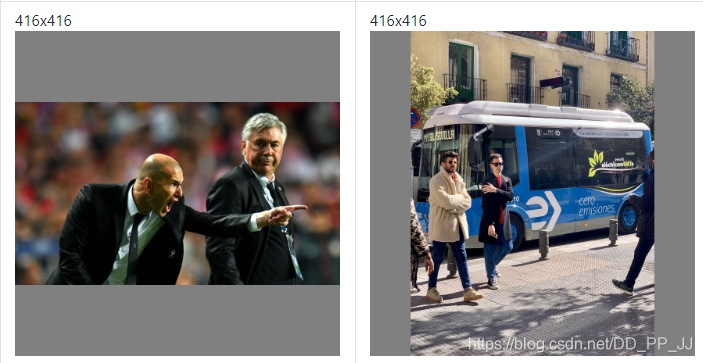
以上就是正方形推理,但是可以看出以上通过补充得到的结果会存在很多冗余信息,而Rectangular Training思路就是想要去掉这些冗余的部分。
具体过程为:求得较长边缩放到416的比例,然后对图片w:h按这个比例缩放,使得较长边达到416,再对较短边进行尽量少的填充使得较短边满足32的倍数。
示例如下:
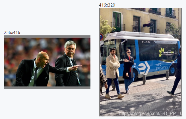
Rectangular Training(矩形训练)
很自然的,训练的过程也可以用到这个想法,减少冗余。不过训练的时候情况比较复杂,由于在训练过程中是一个batch的图片,而每个batch图片是有可能长宽比不同的,这就是与测试最大的区别。具体是实现是取这个batch中最大的场合宽,然后将整个batch中填充到max width和max height,这样操作对小一些的图片来说也是比较浪费。这里的yolov3的实现主要就是优化了一下如何将比例相近的图片放在一个batch,这样显然填充的就更少一些了。作者在issue中提到,在coco数据集中使用这个策略进行训练,能够快⅓。
而如果选择开启矩形训练,必须要关闭dataloader中的shuffle参数,防止对数据的顺序进行调整。同时如果选择image_weights, 根据图片进行采样,也无法与矩阵训练同时使用。
3.2 getitem函数
    def __getitem__(self, index):
        # 新的下角标
        if self.image_weights:
            index = self.indices[index]

        img_path = self.img_files[index]
        label_path = self.label_files[index]

        hyp = self.hyp
        mosaic = True and self.augment
        # 如果开启镶嵌增强、数据增强
        # 加载四张图片,作为一个镶嵌,具体看下文解析。
        if mosaic:
            # 加载镶嵌内容
            img, labels = load_mosaic(self, index)
            shapes = None

        else:
            # 加载图片
            img, (h0, w0), (h, w) = load_image(self, index)

            # 仿射变换
            shape = self.batch_shapes[self.batch[
                index]] if self.rect else self.img_size
            img, ratio, pad = letterbox(img,
                                        shape,
                                        auto=False,
                                        scaleup=self.augment)
            shapes = (h0, w0), (
                (h / h0, w / w0), pad)

            # 加载标注文件
            labels = []
            if os.path.isfile(label_path):
                x = self.labels[index]
                if x is None:  # 如果标签没有加载,读取label_path内容
                    with open(label_path, 'r') as f:
                        x = np.array(
                            [x.split() for x in f.read().splitlines()],
                            dtype=np.float32)

                if x.size > 0:
                    # 将归一化后的xywh转化为左上角、右下角的表达形式
                    labels = x.copy()
                    labels[:, 1] = ratio[0] * w * (
                        x[:, 1] - x[:, 3] / 2) + pad[0]  # pad width
                    labels[:, 2] = ratio[1] * h * (
                        x[:, 2] - x[:, 4] / 2) + pad[1]  # pad height
                    labels[:, 3] = ratio[0] * w * (x[:, 1] +
                                                   x[:, 3] / 2) + pad[0]
                    labels[:, 4] = ratio[1] * h * (x[:, 2] +
                                                   x[:, 4] / 2) + pad[1]

        if self.augment:
            # 图片空间的数据增强
            if not mosaic:
                # 如果没有使用镶嵌的方法,那么对图片进行随机放射
                img, labels = random_affine(img,
                                            labels,
                                            degrees=hyp['degrees'],
                                            translate=hyp['translate'],
                                            scale=hyp['scale'],
                                            shear=hyp['shear'])

            # 增强hsv空间
            augment_hsv(img,
                        hgain=hyp['hsv_h'],
                        sgain=hyp['hsv_s'],
                        vgain=hyp['hsv_v'])

        nL = len(labels)  # 标注文件个数

        if nL:
            # 将 xyxy 格式转化为 xywh 格式
            labels[:, 1:5] = xyxy2xywh(labels[:, 1:5])

            # 归一化到0-1之间
            labels[:, [2, 4]] /= img.shape[0]  # height
            labels[:, [1, 3]] /= img.shape[1]  # width

        if self.augment:
            # 随机左右翻转
            lr_flip = True
            if lr_flip and random.random() < 0.5:
                img = np.fliplr(img)
                if nL:
                    labels[:, 1] = 1 - labels[:, 1]

            # 随机上下翻转
            ud_flip = False
            if ud_flip and random.random() < 0.5:
                img = np.flipud(img)
                if nL:
                    labels[:, 2] = 1 - labels[:, 2]

        labels_out = torch.zeros((nL, 6))
        if nL:
            labels_out[:, 1:] = torch.from_numpy(labels)

        # 图像维度转换
        img = img[:, :, ::-1].transpose(2, 0, 1)  # BGR to RGB, to 3x416x416
        img = np.ascontiguousarray(img)

        return torch.from_numpy(img), labels_out, img_path, shapes
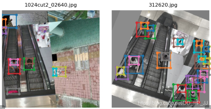
下图是开启了镶嵌和旋转以后的增强效果(mosaic不知道翻译的对不对,如果有问题,欢迎指正。)
这里理解镶嵌就是将四张图片,以不同的比例,合成为一张图片。
3.3 collate_fn函数
    @staticmethod
    def collate_fn(batch):
        img, label, path, shapes = zip(*batch)  # transposed
        for i, l in enumerate(label):
            l[:, 0] = i  # add target image index for build_targets()
        return torch.stack(img, 0), torch.cat(label, 0), path, shapes
还有最后一点内容,是关于pytorch的数据读取机制,本人曾经单纯的认为dataloader仅仅是通过调用__getitem__(self, index),然后就可以直接返回结果。但是之前做过的一个项目打破了这样的认知,在pytorch的dataloader中是会对通过getitem方法得到的结果(batch)进行包装,而这个包装可能与我们想要的有所不同。默认的方法可以看以下代码:
def default_collate(batch):
    r"""Puts each data field into a tensor with outer dimension batch size"""

    elem_type = type(batch[0])
    if isinstance(batch[0], torch.Tensor):
        out = None
        if _use_shared_memory:
            # If we're in a background process, concatenate directly into a
            # shared memory tensor to avoid an extra copy
            numel = sum([x.numel() for x in batch])
            storage = batch[0].storage()._new_shared(numel)
            out = batch[0].new(storage)
        return torch.stack(batch, 0, out=out)
    elif elem_type.__module__ == 'numpy' and elem_type.__name__ != 'str_' \
            and elem_type.__name__ != 'string_':
        elem = batch[0]
        if elem_type.__name__ == 'ndarray':
            # array of string classes and object
            if np_str_obj_array_pattern.search(elem.dtype.str) is not None:
                raise TypeError(error_msg_fmt.format(elem.dtype))

            return default_collate([torch.from_numpy(b) for b in batch])
        if elem.shape == ():  # scalars
            py_type = float if elem.dtype.name.startswith('float') else int
            return numpy_type_map[elem.dtype.name](list(map(py_type, batch)))
    elif isinstance(batch[0], float):
        return torch.tensor(batch, dtype=torch.float64)
    elif isinstance(batch[0], int_classes):
        return torch.tensor(batch)
    elif isinstance(batch[0], string_classes):
        return batch
    elif isinstance(batch[0], container_abcs.Mapping):
        return {key: default_collate([d[key] for d in batch]) for key in batch[0]}
    elif isinstance(batch[0], tuple) and hasattr(batch[0], '_fields'):  # namedtuple
        return type(batch[0])(*(default_collate(samples) for samples in zip(*batch)))
    elif isinstance(batch[0], container_abcs.Sequence):
        transposed = zip(*batch)
        return [default_collate(samples) for samples in transposed]

    raise TypeError((error_msg_fmt.format(type(batch[0]))))
会根据你的数据类型进行相应的处理,但是这往往不是我们需要的,所以需要修改collate_fn,具体内容请看代码,比较简单,就不多赘述。
后记:今天的代码读的比较费力,仅仅通过数据加载这部分就能感受到作者所添加的trick,还有思维的严禁,对数据的限制,处理,都已经提前想好了。不仅如此,作者还添加了巨多的数据增强方法,不仅有传统的仿射变换、上下翻转、左右翻转还有比较新颖的比如镶嵌。以上就是为各位大致理了一遍思路,具体的实现还需要再进行细细的琢磨,不过就使用而言,以上信息就已经足够。由于时间仓促,可能还有一些内容调查的不够严谨,比如说镶嵌这个翻译是否正确,欢迎有这方面了解的大佬与我沟通,期待您的指教。
参考文献
矩形训练相关:https://blog.csdn.net/songwsx/article/details/102639770
仿射变换:https://zhuanlan.zhihu.com/p/93822508
Rectangle Trainning:https://github.com/ultralytics/yolov3/issues/232
数据自由读取:https://zhuanlan.zhihu.com/p/30385675
四、YOLOv3中的参数搜索
前言:YOLOv3代码中也提供了参数搜索,可以为对应的数据集进化一套合适的超参数。本文建档分析一下有关这部分的操作方法以及其参数的具体进化方法。
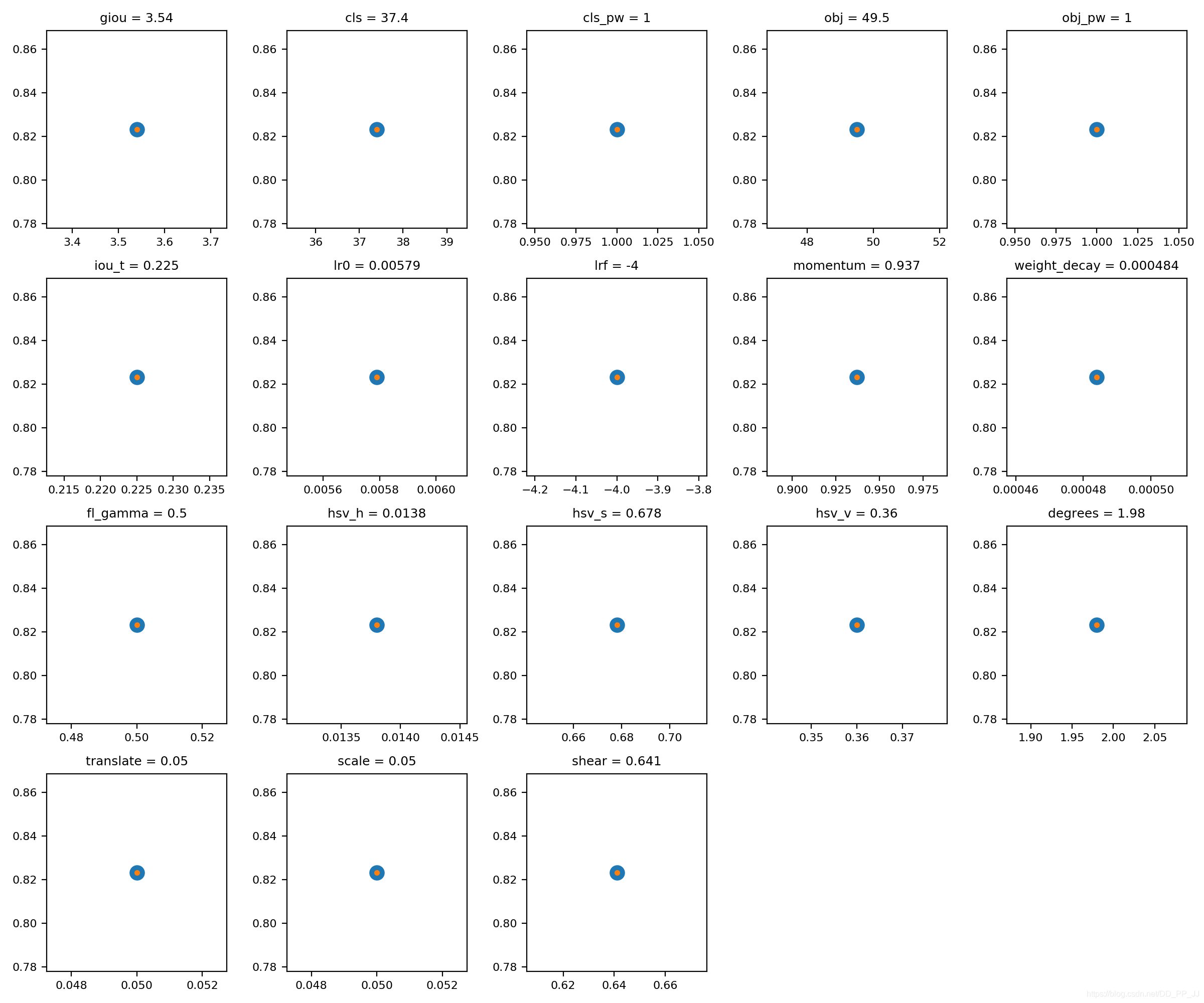
1. 超参数
YOLOv3中的 超参数在train.py中提供,其中包含了一些数据增强参数设置,具体内容如下:
hyp = {'giou': 3.54,  # giou loss gain
       'cls': 37.4,  # cls loss gain
       'cls_pw': 1.0,  # cls BCELoss positive_weight
       'obj': 49.5,  # obj loss gain (*=img_size/320 if img_size != 320)
       'obj_pw': 1.0,  # obj BCELoss positive_weight
       'iou_t': 0.225,  # iou training threshold
       'lr0': 0.00579,  # initial learning rate (SGD=1E-3, Adam=9E-5)
       'lrf': -4.,  # final LambdaLR learning rate = lr0 * (10 ** lrf)
       'momentum': 0.937,  # SGD momentum
       'weight_decay': 0.000484,  # optimizer weight decay
       'fl_gamma': 0.5,  # focal loss gamma
       'hsv_h': 0.0138,  # image HSV-Hue augmentation (fraction)
       'hsv_s': 0.678,  # image HSV-Saturation augmentation (fraction)
       'hsv_v': 0.36,  # image HSV-Value augmentation (fraction)
       'degrees': 1.98,  # image rotation (+/- deg)
       'translate': 0.05,  # image translation (+/- fraction)
       'scale': 0.05,  # image scale (+/- gain)
       'shear': 0.641}  # image shear (+/- deg)
2. 使用方法
在训练的时候,train.py提供了一个可选参数--evolve, 这个参数决定了是否进行超参数搜索与进化(默认是不开启超参数搜索的)。
具体使用方法也很简单:
python train.py --data data/voc.data
                --cfg cfg/yolov3-tiny.cfg
                --img-size 416
                --epochs 273
                --evolve
实际使用的时候,需要进行修改,train.py中的约444行:
for _ in range(1): # generations to evolve
将其中的1修改为你想设置的迭代数,比如200代,如果不设置,结果将会如下图所示,实际上就是只有一代。
3. 原理
整个过程比较简单,对于进化过程中的新一代,都选了了适应性最高的前一代(在前几代中)进行突变。以上所有的参数将有约20%的 1-sigma的正态分布几率同时突变。
s = 0.2 # sigma
整个进化过程需要搞清楚两个点:
- 如何评判其中一代的好坏?
- 下一代如何根据上一代进行进化?
第一个问题:判断好坏的标准。
def fitness(x):
    w = [0.0, 0.0, 0.8, 0.2]
    # weights for [P, R, mAP, F1]@0.5
    return (x[:, :4] * w).sum(1)
YOLOv3进化部分是通过以上的适应度函数判断的,适应度越高,代表这一代的性能越好。而在适应度中,是通过Precision,Recall ,mAP,F1这四个指标作为适应度的评价标准。
其中的w是设置的加权,如果更关心mAP的值,可以提高mAP的权重;如果更关心F1,则设置更高的权重在对应的F1上。这里分配mAP权重为0.8、F1权重为0.2。
第二个问题:如何进行进化?
进化过程中有两个重要的参数:
第一个参数为parent, 可选值为single或者weighted,这个参数的作用是:决定如何选择上一代。如果选择single,代表只选择上一代中最好的那个。
 if parent == 'single' or len(x) == 1:
    x = x[fitness(x).argmax()]
如果选择weighted,代表选择得分的前10个加权平均的结果作为下一代,具体操作如下:
elif parent == 'weighted':  # weighted combination
    n = min(10, len(x))  # number to merge
    x = x[np.argsort(-fitness(x))][:n]  # top n mutations
    w = fitness(x) - fitness(x).min()  # weights
    x = (x * w.reshape(n, 1)).sum(0) / w.sum()  # new parent
第二个参数为method,可选值为1,2,3, 分别代表使用三种模式来进化:
# Mutate
method = 2
s = 0.2  # 20% sigma
np.random.seed(int(time.time()))
g = np.array([1, 1, 1, 1, 1, 1, 1, 0, .1, \
              1, 0, 1, 1, 1, 1, 1, 1, 1])  # gains
# 这里的g类似加权
ng = len(g)
if method == 1:
    v = (np.random.randn(ng) *
         np.random.random() * g * s + 1) ** 2.0
elif method == 2:
    v = (np.random.randn(ng) *
         np.random.random(ng) * g * s + 1) ** 2.0
elif method == 3:
    v = np.ones(ng)
    while all(v == 1):
        # 为了防止重复,直到有变化才停下来
         r = (np.random.random(ng) < 0.1) * np.random.randn(ng)
         # 10% 的突变几率
         v = (g * s * r + 1) ** 2.0

for i, k in enumerate(hyp.keys()):
    hyp[k] = x[i + 7] * v[i]
    # 进行突变
另外,为了防止突变过程,导致参数出现明显不合理的范围,需要用一个范围进行框定,将超出范围的内容剪切掉。具体方法如下:
# Clip to limits
keys = ['lr0', 'iou_t', 'momentum',
        'weight_decay', 'hsv_s',
        'hsv_v', 'translate',
        'scale', 'fl_gamma']
limits = [(1e-5, 1e-2), (0.00, 0.70),
          (0.60, 0.98), (0, 0.001),
          (0, .9), (0, .9), (0, .9),
          (0, .9), (0, 3)]

for k, v in zip(keys, limits):
    hyp[k] = np.clip(hyp[k], v[0], v[1])
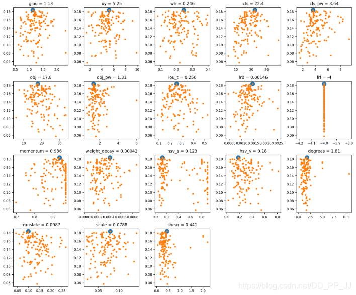
最终训练的超参数搜索的结果可视化:
参考资料:
官方issue: https://github.com/ultralytics/yolov3/issues/392
官方代码:https://github.com/ultralytics/yolov3
五、网络模型的构建
前言:之前几篇讲了cfg文件的理解、数据集的构建、数据加载机制和超参数进化机制,本文将讲解YOLOv3如何从cfg文件构造模型。本文涉及到一个比较有用的部分就是bias的设置,可以提升mAP、F1、P、R等指标,还能让训练过程更加平滑。
1. cfg文件
在YOLOv3中,修改网络结构很容易,只需要修改cfg文件即可。目前,cfg文件支持convolutional, maxpool, unsample, route, shortcut, yolo这几个层。
而且作者也提供了多个cfg文件来进行网络构建,比如:yolov3.cfg、yolov3-tiny.cfg、yolov3-spp.cfg、csresnext50-panet-spp.cfg文件(提供的yolov3-spp-pan-scale.cfg文件,在代码级别还没有提供支持)。
如果想要添加自定义的模块也很方便,比如说注意力机制模块、空洞卷积等,都可以简单地得到添加或者修改。
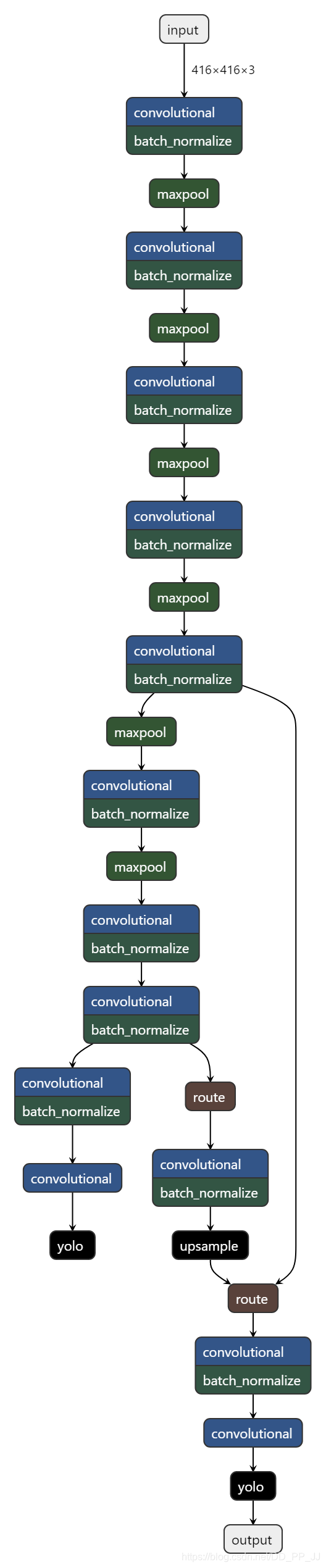
为了更加方便的理解cfg文件网络是如何构建的,在这里推荐一个Github上的网络结构可视化软件:Netron,下图是可视化yolov3-tiny的结果:
2. 网络模型构建
从train.py文件入手,其中涉及的网络构建的代码为:
# Initialize model
model = Darknet(cfg, arc=opt.arc).to(device)
然后沿着Darknet实现进行讲解:
class Darknet(nn.Module):
    # YOLOv3 object detection model
    def __init__(self, cfg, img_size=(416, 416), arc='default'):
        super(Darknet, self).__init__()
        self.module_defs = parse_model_cfg(cfg)
        self.module_list, self.routs = create_modules(self.module_defs, img_size, arc)
        self.yolo_layers = get_yolo_layers(self)

        # Darknet Header
        self.version = np.array([0, 2, 5], dtype=np.int32)
        # (int32) version info: major, minor, revision
        self.seen = np.array([0], dtype=np.int64)
        # (int64) number of images seen during training
以上文件中,比较关键的就是成员函变量module_defs、module_list、routs、yolo_layers四个成员函数,先对这几个参数的意义进行解释:
2.1 module_defs
调用了parse_model_cfg函数,得到了module_defs对象。实际上该函数是通过解析cfg文件,得到一个list,list中包含多个字典,每个字典保存的内容就是一个模块内容,比如说:
[convolutional]
batch_normalize=1
filters=128
size=3
stride=2
pad=1
activation=leaky
函数代码如下:
def parse_model_cfg(path):
    # path参数为: cfg/yolov3-tiny.cfg
    if not path.endswith('.cfg'):
        path += '.cfg'
    if not os.path.exists(path) and os.path.exists('cfg' + os.sep + path):
        path = 'cfg' + os.sep + path

    with open(path, 'r') as f:
        lines = f.read().split('\n')

    # 去除以#开头的,属于注释部分的内容
    lines = [x for x in lines if x and not x.startswith('#')]
    lines = [x.rstrip().lstrip() for x in lines]
    mdefs = []  # 模块的定义
    for line in lines:
        if line.startswith('['):  # 标志着一个模块的开始
            '''
            比如:
            [shortcut]
            from=-3
            activation=linear
            '''
            mdefs.append({})
            mdefs[-1]['type'] = line[1:-1].rstrip()
            if mdefs[-1]['type'] == 'convolutional':
                mdefs[-1]['batch_normalize'] = 0
                # pre-populate with zeros (may be overwritten later)
        else:
            # 将键和键值放入字典
            key, val = line.split("=")
            key = key.rstrip()

            if 'anchors' in key:
                mdefs[-1][key] = np.array([float(x) for x in val.split(',')]).reshape((-1, 2))  # np anchors
            else:
                mdefs[-1][key] = val.strip()

    # 支持的参数类型
    supported = ['type', 'batch_normalize', 'filters', 'size',\
                 'stride', 'pad', 'activation', 'layers', 'groups',\
                 'from', 'mask', 'anchors', 'classes', 'num', 'jitter', \
                 'ignore_thresh', 'truth_thresh', 'random',\
                 'stride_x', 'stride_y']

    # 判断所有参数中是否有不符合要求的key
    f = []
    for x in mdefs[1:]:
        [f.append(k) for k in x if k not in f]
    u = [x for x in f if x not in supported]  # unsupported fields
    assert not any(u), "Unsupported fields %s in %s. See https://github.com/ultralytics/yolov3/issues/631" % (u, path)

    return mdefs
返回的内容通过debug模式进行查看:
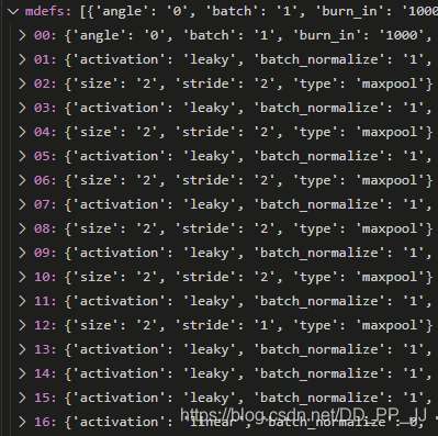
其中需要关注的就是anchor的组织:
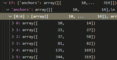
可以看出,anchor是按照每两个一对进行组织的,与我们的理解一致。
2.2 module_list&routs
这个部分是本文的核心,也是理解模型构建的关键。
在pytorch中,构建模型常见的有通过Sequential或者ModuleList进行构建。
通过Sequential构建
model=nn.Sequential()
model.add_module('conv',nn.Conv2d(3,3,3))
model.add_module('batchnorm',nn.BatchNorm2d(3))
model.add_module('activation_layer',nn.ReLU())
或者
model=nn.Sequential(
    nn.Conv2d(3,3,3),
    nn.BatchNorm2d(3),
    nn.ReLU()
    )
或者
from collections import OrderedDict
model=nn.Sequential(OrderedDict([
    ('conv',nn.Conv2d(3,3,3)),
    ('batchnorm',nn.BatchNorm2d(3)),
    ('activation_layer',nn.ReLU())
]))
通过sequential构建的模块内部实现了forward函数,可以直接传入参数,进行调用。
通过ModuleList构建
model=nn.ModuleList([nn.Linear(3,4),
                         nn.ReLU(),
                         nn.Linear(4,2)])
ModuleList类似list,内部没有实现forward函数,使用的时候需要构建forward函数,构建自己模型常用ModuleList函数建立子模型,建立forward函数实现前向传播。
在YOLOv3中,灵活地结合了两种使用方式,通过解析以上得到的module_defs,进行构建一个ModuleList,然后再通过构建forward函数进行前向传播即可。
具体代码如下:
def create_modules(module_defs, img_size, arc):
# 通过module_defs进行构建模型
hyperparams = module_defs.pop(0)
output_filters = [int(hyperparams['channels'])]
module_list = nn.ModuleList()
routs = [] # 存储了所有的层,在route、shortcut会使用到。
yolo_index = -1
for i, mdef in enumerate(module_defs):
modules = nn.Sequential()
'''
通过type字样不同的类型,来进行模型构建
'''
if mdef['type'] == 'convolutional':
bn = int(mdef['batch_normalize'])
filters = int(mdef['filters'])
size = int(mdef['size'])
stride = int(mdef['stride']) if 'stride' in mdef else (int(
mdef['stride_y']), int(mdef['stride_x']))
pad = (size - 1) // 2 if int(mdef['pad']) else 0
modules.add_module(
'Conv2d',
nn.Conv2d(
in_channels=output_filters[-1],
out_channels=filters,
kernel_size=size,
stride=stride,
padding=pad,
groups=int(mdef['groups']) if 'groups' in mdef else 1,
bias=not bn))
if bn:
modules.add_module('BatchNorm2d',
nn.BatchNorm2d(filters, momentum=0.1))
if mdef['activation'] == 'leaky': # TODO: activation study https://github.com/ultralytics/yolov3/issues/441
modules.add_module('activation', nn.LeakyReLU(0.1,
inplace=True))
elif mdef['activation'] == 'swish':
modules.add_module('activation', Swish())
# 在此处可以添加新的激活函数
elif mdef['type'] == 'maxpool':
# 最大池化操作
size = int(mdef['size'])
stride = int(mdef['stride'])
maxpool = nn.MaxPool2d(kernel_size=size,
stride=stride,
padding=int((size - 1) // 2))
if size == 2 and stride == 1: # yolov3-tiny
modules.add_module('ZeroPad2d', nn.ZeroPad2d((0, 1, 0, 1)))
modules.add_module('MaxPool2d', maxpool)
else:
modules = maxpool
elif mdef['type'] == 'upsample':
# 通过近邻插值完成上采样
modules = nn.Upsample(scale_factor=int(mdef['stride']),
mode='nearest')
elif mdef['type'] == 'route':
# nn.Sequential() placeholder for 'route' layer
layers = [int(x) for x in mdef['layers'].split(',')]
filters = sum(
[output_filters[i + 1 if i > 0 else i] for i in layers])
# extend表示添加一系列对象
routs.extend([l if l > 0 else l + i for l in layers])
elif mdef['type'] == 'shortcut':
# nn.Sequential() placeholder for 'shortcut' layer
filters = output_filters[int(mdef['from'])]
layer = int(mdef['from'])
routs.extend([i + layer if layer < 0 else layer])
elif mdef['type'] == 'yolo':
yolo_index += 1
mask = [int(x) for x in mdef['mask'].split(',')] # anchor mask
modules = YOLOLayer(
anchors=mdef['anchors'][mask], # anchor list
nc=int(mdef['classes']), # number of classes
img_size=img_size, # (416, 416)
yolo_index=yolo_index, # 0, 1 or 2
arc=arc) # yolo architecture
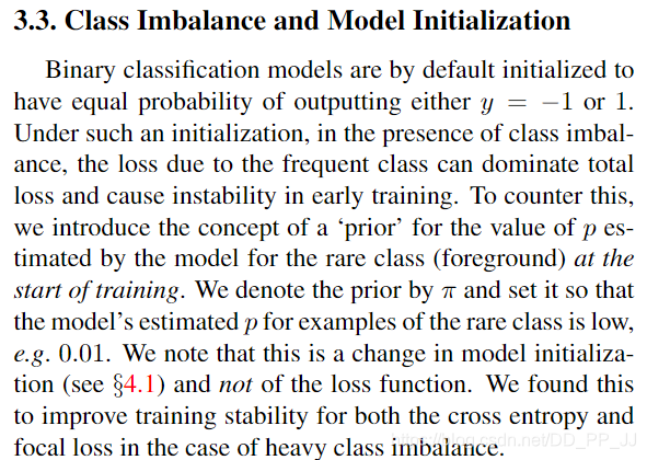
# 这是在focal loss文章中提到的为卷积层添加bias
# 主要用于解决样本不平衡问题
# (论文地址 https://arxiv.org/pdf/1708.02002.pdf section 3.3)
# 具体讲解见下方
try:
if arc == 'defaultpw' or arc == 'Fdefaultpw':
# default with positive weights
b = [-5.0, -5.0] # obj, cls
elif arc == 'default':
# default no pw (40 cls, 80 obj)
b = [-5.0, -5.0]
elif arc == 'uBCE':
# unified BCE (80 classes)
b = [0, -9.0]
elif arc == 'uCE':
# unified CE (1 background + 80 classes)
b = [10, -0.1]
elif arc == 'Fdefault':
# Focal default no pw (28 cls, 21 obj, no pw)
b = [-2.1, -1.8]
elif arc == 'uFBCE' or arc == 'uFBCEpw':
# unified FocalBCE (5120 obj, 80 classes)
b = [0, -6.5]
elif arc == 'uFCE':
# unified FocalCE (64 cls, 1 background + 80 classes)
b = [7.7, -1.1]
bias = module_list[-1][0].bias.view(len(mask), -1)
# 255 to 3x85
bias[:, 4] += b[0] - bias[:, 4].mean() # obj
bias[:, 5:] += b[1] - bias[:, 5:].mean() # cls
# 将新的偏移量赋值回模型中
module_list[-1][0].bias = torch.nn.Parameter(bias.view(-1))
except:
print('WARNING: smart bias initialization failure.')
else:
print('Warning: Unrecognized Layer Type: ' + mdef['type'])
# 将module内容保存在module_list中。
module_list.append(modules)
# 保存所有的filter个数
output_filters.append(filters)
return module_list, routs
bias部分讲解
其中在YOLO Layer部分涉及到一个初始化的trick,来自Focal Loss中关于模型初始化的讨论,具体内容请阅读论文,https://arxiv.org/pdf/1708.02002.pdf 的第3.3节。
这里涉及到一个非常insight的点,笔者与BBuf讨论了很长时间,才理解这样做的原因。
我们在第一篇中介绍了,YOLO层前一个卷积的filter个数计算公式如下:
5代表x,y,w,h, score,score代表该格子中是否存在目标,3代表这个格子中会分配3个anchor进行匹配。在YOLOLayer中的forward函数中,有以下代码,需要通过sigmoid激活函数:
if 'default' in self.arc:  # seperate obj and cls
    torch.sigmoid_(io[..., 4])
elif 'BCE' in self.arc:  # unified BCE (80 classes)
    torch.sigmoid_(io[..., 5:])
    io[..., 4] = 1
elif 'CE' in self.arc:  # unified CE (1 background + 80 classes)
    io[..., 4:] = F.softmax(io[..., 4:], dim=4)
    io[..., 4] = 1
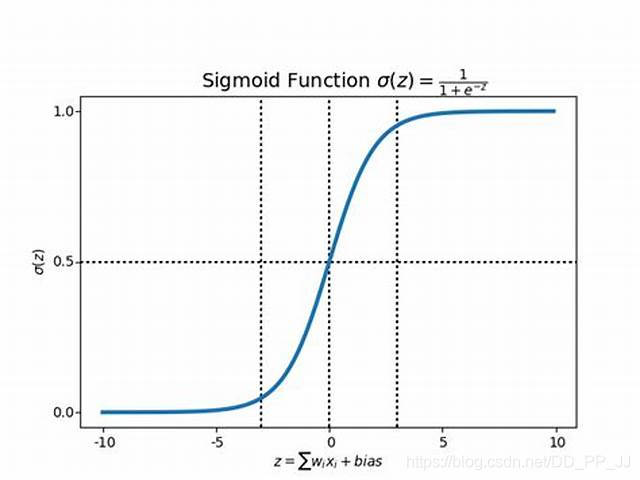
可以观察到,Sigmoid梯度是有限的,大致在[-10,10]之间。
在pytorch中的卷积层默认的初始化是以0为中心点的正态分布,这样进行的初始化会导致很多gird中大约一半得到了激活,在计算loss的时候就会计算上所有的激活的点对应的坐标信息,这样计算loss就会变得很大。
根据这个现象,作者选择在YOLOLayer的前一个卷积层添加bias,来避免这种情况,实际操作就是在原有的bias上减去5,这样通过卷积得到的数值就不会被激活,可以防止在初始阶段的第一个batch中就进行过拟合。通过以上操作,能够让所有的神经元在前几个batch中输出空的检测。
经过作者的实验,通过使用bias的trick,可以提升mAP、F1、P、R等指标,还能让训练过程更加平滑。
2.3 yolo_layers
代码如下:
def get_yolo_layers(model):
    return [i for i, x in enumerate(model.module_defs) if x['type'] == 'yolo']
    # [82, 94, 106] for yolov3
yolo layer的获取是通过解析module_defs这个存储cfg文件中的信息的变量得到的。以yolov3.cfg为例,最终返回的是yolo层在整个module的序号。比如:第83,94,106个层是YOLO层。
3. forward函数
在YOLO中,如果能理解前向传播的过程,那整个网络的构建也就很清楚明了了。
    def forward(self, x, var=None):
        img_size = x.shape[-2:]
        layer_outputs = []
        output = []

        for i, (mdef,
                module) in enumerate(zip(self.module_defs, self.module_list)):
            mtype = mdef['type']
            if mtype in ['convolutional', 'upsample', 'maxpool']:
                # 卷积层,上采样,池化层只需要经过即可
                x = module(x)
            elif mtype == 'route':
                # route操作就是将几个层的内容拼接起来,具体可以看cfg文件解析
                layers = [int(x) for x in mdef['layers'].split(',')]
                if len(layers) == 1:
                    x = layer_outputs[layers[0]]
                else:
                    try:
                        x = torch.cat([layer_outputs[i] for i in layers], 1)
                    except:
                        # apply stride 2 for darknet reorg layer
                        layer_outputs[layers[1]] = F.interpolate(
                            layer_outputs[layers[1]], scale_factor=[0.5, 0.5])
                        x = torch.cat([layer_outputs[i] for i in layers], 1)

            elif mtype == 'shortcut':
                x = x + layer_outputs[int(mdef['from'])]
            elif mtype == 'yolo':
                output.append(module(x, img_size))
            #记录route对应的层
            layer_outputs.append(x if i in self.routs else [])

        if self.training:
            # 如果训练,直接输出YOLO要求的Tensor
            # 3*(class+5)
            return output

        elif ONNX_EXPORT:# 这个是对应的onnx导出的内容
            x = [torch.cat(x, 0) for x in zip(*output)]
            return x[0], torch.cat(x[1:3], 1)  # scores, boxes: 3780x80, 3780x4
        else:
            # 对应测试阶段
            io, p = list(zip(*output))  # inference output, training output
            return torch.cat(io, 1), p
forward的过程也比较简单,通过得到的module_defs和module_list变量,通过for循环将整个module_list中的内容进行一遍串联,需要得到的最终结果是YOLO层的输出。(ps:下一篇文章再进行YOLOLayer的代码解析)
参考资料
sequential用法https://blog.csdn.net/happyday_d/article/details/85629119
https://arxiv.org/pdf/1708.02002.pdf
六、模型构建中的YOLOLayer
前言:上次讲了YOLOv3中的模型构建,从头到尾理了一遍从cfg读取到模型整个构建的过程。其中模型构建中最重要的YOLOLayer还没有梳理,本文将从代码的角度理解YOLOLayer的构建与实现。
1. Grid创建
YOLOv3是一个单阶段的目标检测器,将目标划分为不同的grid,每个grid分配3个anchor作为先验框来进行匹配。首先读一下代码中关于grid创建的部分。
首先了解一下pytorch中的API:torch.mershgrid
举一个简单的例子就比较清楚了:
Python 3.7.3 (default, Apr 24 2019, 15:29:51) [MSC v.1915 64 bit (AMD64)] :: Anaconda, Inc. on win32
Type "help", "copyright", "credits" or "license" for more information.
>>> import torch
>>> a = torch.arange(3)
>>> b = torch.arange(5)
>>> x,y = torch.meshgrid(a,b)
>>> a
tensor([0, 1, 2])
>>> b
tensor([0, 1, 2, 3, 4])
>>> x
tensor([[0, 0, 0, 0, 0],
        [1, 1, 1, 1, 1],
        [2, 2, 2, 2, 2]])
>>> y
tensor([[0, 1, 2, 3, 4],
        [0, 1, 2, 3, 4],
        [0, 1, 2, 3, 4]])
>>>
单纯看输入输出,可能不是很明白,列举一个例子:
>>> for i in range(3):
...     for j in range(4):
...         print("(", x[i,j], "," ,y[i,j],")")
...
( tensor(0) , tensor(0) )
( tensor(0) , tensor(1) )
( tensor(0) , tensor(2) )
( tensor(0) , tensor(3) )
( tensor(1) , tensor(0) )
( tensor(1) , tensor(1) )
( tensor(1) , tensor(2) )
( tensor(1) , tensor(3) )
( tensor(2) , tensor(0) )
( tensor(2) , tensor(1) )
( tensor(2) , tensor(2) )
( tensor(2) , tensor(3) )

>>> torch.stack((x,y),2)
tensor([[[0, 0],
         [0, 1],
         [0, 2],
         [0, 3],
         [0, 4]],

        [[1, 0],
         [1, 1],
         [1, 2],
         [1, 3],
         [1, 4]],

        [[2, 0],
         [2, 1],
         [2, 2],
         [2, 3],
         [2, 4]]])
>>>
现在就比较清楚了,划分了3×4的网格,通过遍历得到的x和y就能遍历全部格子。
下面是yolov3中提供的代码(需要注意的是这是针对某一层YOLOLayer,而不是所有的YOLOLayer):
def create_grids(self,
                 img_size=416,
                 ng=(13, 13),
                 device='cpu',
                 type=torch.float32):
    nx, ny = ng  # 网格尺寸
    self.img_size = max(img_size)
    #下采样倍数为32
    self.stride = self.img_size / max(ng)

    # 划分网格,构建相对左上角的偏移量
    yv, xv = torch.meshgrid([torch.arange(ny), torch.arange(nx)])
    # 通过以上例子很容易理解
    self.grid_xy = torch.stack((xv, yv), 2).to(device).type(type).view(
        (1, 1, ny, nx, 2))

    # 处理anchor,将其除以下采样倍数
    self.anchor_vec = self.anchors.to(device) / self.stride
    self.anchor_wh = self.anchor_vec.view(1, self.na, 1, 1,
                                          2).to(device).type(type)
    self.ng = torch.Tensor(ng).to(device)
    self.nx = nx
    self.ny = ny
2. YOLOLayer
在之前的文章中讲过,YOLO层前一层卷积层的filter个数具有特殊的要求,计算方法为:
如下图所示:
训练过程:
YOLOLayer的作用就是对上一个卷积层得到的张量进行处理,具体可以看training过程涉及的代码(暂时不关心ONNX部分的代码):
class YOLOLayer(nn.Module):
def __init__(self, anchors, nc, img_size, yolo_index, arc):
super(YOLOLayer, self).__init__()
self.anchors = torch.Tensor(anchors)
self.na = len(anchors) # 该YOLOLayer分配给每个grid的anchor的个数
self.nc = nc # 类别个数
self.no = nc + 5 # 每个格子对应输出的维度 class + 5 中5代表x,y,w,h,conf
self.nx = 0 # 初始化x方向上的格子数量
self.ny = 0 # 初始化y方向上的格子数量
self.arc = arc
if ONNX_EXPORT: # grids must be computed in __init__
stride = [32, 16, 8][yolo_index] # stride of this layer
nx = int(img_size[1] / stride) # number x grid points
ny = int(img_size[0] / stride) # number y grid points
create_grids(self, img_size, (nx, ny))
def forward(self, p, img_size, var=None):
'''
onnx代表开放式神经网络交换
pytorch中的模型都可以导出或转换为标准ONNX格式
在模型采用ONNX格式后,即可在各种平台和设备上运行
在这里ONNX代表规范化的推理过程
'''
if ONNX_EXPORT:
bs = 1 # batch size
else:
bs, _, ny, nx = p.shape # bs, 255, 13, 13
if (self.nx, self.ny) != (nx, ny):
create_grids(self, img_size, (nx, ny), p.device, p.dtype)
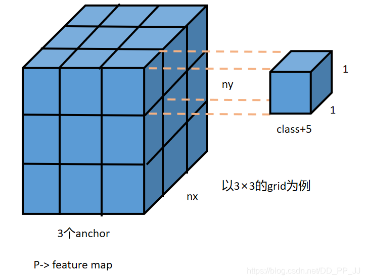
# p.view(bs, 255, 13, 13) -- > (bs, 3, 13, 13, 85)
# (bs, anchors, grid, grid, classes + xywh)
p = p.view(bs, self.na, self.no, self.ny,
self.nx).permute(0, 1, 3, 4, 2).contiguous()
if self.training:
return p
在理解以上代码的时候,需要理解每一个通道所代表的意义,原先的P是由上一层卷积得到的feature map, 形状为(以80个类别、输入416、下采样32倍为例):【batch size, anchor×(80+5), 13, 13】,在训练的过程中,将feature map通过张量操作转化的形状为:【batch size, anchor, 13, 13, 85】。
测试过程:
# p的形状目前为:【bs, anchor_num, gridx,gridy,xywhc+class】
else:  # 测试推理过程
    # s = 1.5  # scale_xy  (pxy = pxy * s - (s - 1) / 2)
    io = p.clone()  # 测试过程输出就是io
    io[..., :2] = torch.sigmoid(io[..., :2]) + self.grid_xy  # xy
    # grid_xy是左上角再加上偏移量io[...:2]代表xy偏移
    io[..., 2:4] = torch.exp(
        io[..., 2:4]) * self.anchor_wh  # wh yolo method
    # io[..., 2:4] = ((torch.sigmoid(io[..., 2:4]) * 2) ** 3) * self.anchor_wh
    # wh power method
    io[..., :4] *= self.stride

    if 'default' in self.arc:  # seperate obj and cls
        torch.sigmoid_(io[..., 4])
    elif 'BCE' in self.arc:  # unified BCE (80 classes)
        torch.sigmoid_(io[..., 5:])
        io[..., 4] = 1
    elif 'CE' in self.arc:  # unified CE (1 background + 80 classes)
        io[..., 4:] = F.softmax(io[..., 4:], dim=4)
        io[..., 4] = 1

    if self.nc == 1:
        io[..., 5] = 1
        # single-class model https://github.com/ultralytics/yolov3/issues/235

    # reshape from [1, 3, 13, 13, 85] to [1, 507, 85]
    return io.view(bs, -1, self.no), p
理解以上内容是需要对应以下公式:
xy部分:
c_x, c_y代表的是格子的左上角坐标;t_x, t_y代表的是网络预测的结果;\sigma代表sigmoid激活函数。对应代码理解:
io[..., :2] = torch.sigmoid(io[..., :2]) + self.grid_xy  # xy
# grid_xy是左上角再加上偏移量io[...:2]代表xy偏移
wh部分:
p_w, p_h代表的是anchor先验框在feature map上对应的大小。t_w, t_h代表的是网络学习得到的缩放系数。对应代码理解:
# wh yolo method
io[..., 2:4] = torch.exp(io[..., 2:4]) * self.anchor_wh
class部分:
在类别部分,提供了几种方法,根据arc参数来进行不同模式的选择。以CE(crossEntropy)为例:
#io: (bs, anchors, grid, grid, xywh+classes)
io[..., 4:] = F.softmax(io[..., 4:], dim=4)# 使用softmax
io[..., 4] = 1
3. 参考资料
pytorch的官方API
输出解码:https://zhuanlan.zhihu.com/p/76802514
七、在YOLOv3模型中添加Attention机制
前言:【从零开始学习YOLOv3】系列越写越多,本来安排的内容比较少,但是在阅读代码的过程中慢慢发掘了一些新的亮点,所以不断加入到这个系列中。之前都在读YOLOv3中的代码,已经学习了cfg文件、模型构建等内容。本文在之前的基础上,对模型的代码进行修改,将之前Attention系列中的SE模块和CBAM模块集成到YOLOv3中。
1. 规定格式
正如[convolutional],[maxpool],[net],[route]等层在cfg中的定义一样,我们再添加全新的模块的时候,要规定一下cfg的格式。做出以下规定:
在SE模块(具体讲解见: 【cv中的Attention机制】最简单最易实现的SE模块)中,有一个参数为reduction,这个参数默认是16,所以在这个模块中的详细参数我们按照以下内容进行设置:
[se]
reduction=16
在CBAM模块(具体讲解见: 【CV中的Attention机制】ECCV 2018 Convolutional Block Attention Module)中,空间注意力机制和通道注意力机制中一共存在两个参数:ratio和kernel_size, 所以这样规定CBAM在cfg文件中的格式:
[cbam]
ratio=16
kernelsize=7
2. 修改解析部分
由于我们添加的这些参数都是自定义的,所以需要修改解析cfg文件的函数,之前讲过,需要修改parse_config.py中的部分内容:
def parse_model_cfg(path):
    # path参数为: cfg/yolov3-tiny.cfg
    if not path.endswith('.cfg'):
        path += '.cfg'
    if not os.path.exists(path) and \
           os.path.exists('cfg' + os.sep + path):
        path = 'cfg' + os.sep + path

    with open(path, 'r') as f:
        lines = f.read().split('\n')

    # 去除以#开头的,属于注释部分的内容
    lines = [x for x in lines if x and not x.startswith('#')]
    lines = [x.rstrip().lstrip() for x in lines]
    mdefs = []  # 模块的定义
    for line in lines:
        if line.startswith('['):  # 标志着一个模块的开始
            '''
            eg:
            [shortcut]
            from=-3
            activation=linear
            '''
            mdefs.append({})
            mdefs[-1]['type'] = line[1:-1].rstrip()
            if mdefs[-1]['type'] == 'convolutional':
                mdefs[-1]['batch_normalize'] = 0
        else:
            key, val = line.split("=")
            key = key.rstrip()

            if 'anchors' in key:
                mdefs[-1][key] = np.array([float(x) for x in val.split(',')]).reshape((-1, 2))
            else:
                mdefs[-1][key] = val.strip()

    # Check all fields are supported
    supported = ['type', 'batch_normalize', 'filters', 'size',\
                 'stride', 'pad', 'activation', 'layers', \
                 'groups','from', 'mask', 'anchors', \
                 'classes', 'num', 'jitter', 'ignore_thresh',\
                 'truth_thresh', 'random',\
                 'stride_x', 'stride_y']

    f = []  # fields
    for x in mdefs[1:]:
        [f.append(k) for k in x if k not in f]
    u = [x for x in f if x not in supported]  # unsupported fields
    assert not any(u), "Unsupported fields %s in %s. See https://github.com/ultralytics/yolov3/issues/631" % (u, path)

    return mdefs
以上内容中,需要改的是supported中的字段,将我们的内容添加进去:
supported = ['type', 'batch_normalize', 'filters', 'size',\
            'stride', 'pad', 'activation', 'layers', \
            'groups','from', 'mask', 'anchors', \
            'classes', 'num', 'jitter', 'ignore_thresh',\
            'truth_thresh', 'random',\
            'stride_x', 'stride_y',\
            'ratio', 'reduction', 'kernelsize']
3. 实现SE和CBAM
具体原理还请见【cv中的Attention机制】最简单最易实现的SE模块和【CV中的Attention机制】ECCV 2018 Convolutional Block Attention Module这两篇文章,下边直接使用以上两篇文章中的代码:
SE
class SELayer(nn.Module):
    def __init__(self, channel, reduction=16):
        super(SELayer, self).__init__()
        self.avg_pool = nn.AdaptiveAvgPool2d(1)
        self.fc = nn.Sequential(
            nn.Linear(channel, channel // reduction, bias=False),
            nn.ReLU(inplace=True),
            nn.Linear(channel // reduction, channel, bias=False),
            nn.Sigmoid()
        )

    def forward(self, x):
        b, c, _, _ = x.size()
        y = self.avg_pool(x).view(b, c)
        y = self.fc(y).view(b, c, 1, 1)
        return x * y.expand_as(x)
CBAM
class SpatialAttention(nn.Module):
    def __init__(self, kernel_size=7):
        super(SpatialAttention, self).__init__()
        assert kernel_size in (3,7), "kernel size must be 3 or 7"
        padding = 3if kernel_size == 7else1

        self.conv = nn.Conv2d(2,1,kernel_size, padding=padding, bias=False)
        self.sigmoid = nn.Sigmoid()

    def forward(self, x):
        avgout = torch.mean(x, dim=1, keepdim=True)
        maxout, _ = torch.max(x, dim=1, keepdim=True)
        x = torch.cat([avgout, maxout], dim=1)
        x = self.conv(x)
        return self.sigmoid(x)

class ChannelAttention(nn.Module):
    def __init__(self, in_planes, rotio=16):
        super(ChannelAttention, self).__init__()
        self.avg_pool = nn.AdaptiveAvgPool2d(1)
        self.max_pool = nn.AdaptiveMaxPool2d(1)

        self.sharedMLP = nn.Sequential(
            nn.Conv2d(in_planes, in_planes // ratio, 1, bias=False), nn.ReLU(),
            nn.Conv2d(in_planes // rotio, in_planes, 1, bias=False))
        self.sigmoid = nn.Sigmoid()

    def forward(self, x):
        avgout = self.sharedMLP(self.avg_pool(x))
        maxout = self.sharedMLP(self.max_pool(x))
        return self.sigmoid(avgout + maxout)
以上就是两个模块的代码,添加到models.py文件中。
4. 设计cfg文件
这里以yolov3-tiny.cfg为baseline,然后添加注意力机制模块。
CBAM与SE类似,所以以SE为例,添加到backbone之后的部分,进行信息重构(refinement)。
[net]
# Testing
batch=1
subdivisions=1
# Training
# batch=64
# subdivisions=2
width=416
height=416
channels=3
momentum=0.9
decay=0.0005
angle=0
saturation = 1.5
exposure = 1.5
hue=.1

learning_rate=0.001
burn_in=1000
max_batches = 500200
policy=steps
steps=400000,450000
scales=.1,.1

[convolutional]
batch_normalize=1
filters=16
size=3
stride=1
pad=1
activation=leaky

[maxpool]
size=2
stride=2

[convolutional]
batch_normalize=1
filters=32
size=3
stride=1
pad=1
activation=leaky

[maxpool]
size=2
stride=2

[convolutional]
batch_normalize=1
filters=64
size=3
stride=1
pad=1
activation=leaky

[maxpool]
size=2
stride=2

[convolutional]
batch_normalize=1
filters=128
size=3
stride=1
pad=1
activation=leaky

[maxpool]
size=2
stride=2

[convolutional]
batch_normalize=1
filters=256
size=3
stride=1
pad=1
activation=leaky

[maxpool]
size=2
stride=2

[convolutional]
batch_normalize=1
filters=512
size=3
stride=1
pad=1
activation=leaky

[maxpool]
size=2
stride=1

[convolutional]
batch_normalize=1
filters=1024
size=3
stride=1
pad=1
activation=leaky

[se]
reduction=16

# 在backbone结束的地方添加se模块
#####backbone######

[convolutional]
batch_normalize=1
filters=256
size=1
stride=1
pad=1
activation=leaky

[convolutional]
batch_normalize=1
filters=512
size=3
stride=1
pad=1
activation=leaky

[convolutional]
size=1
stride=1
pad=1
filters=18
activation=linear


[yolo]
mask = 3,4,5
anchors = 10,14,  23,27,  37,58,  81,82,  135,169,  344,319
classes=1
num=6
jitter=.3
ignore_thresh = .7
truth_thresh = 1
random=1

[route]
layers = -4

[convolutional]
batch_normalize=1
filters=128
size=1
stride=1
pad=1
activation=leaky

[upsample]
stride=2

[route]
layers = -1, 8

[convolutional]
batch_normalize=1
filters=256
size=3
stride=1
pad=1
activation=leaky

[convolutional]
size=1
stride=1
pad=1
filters=18
activation=linear

[yolo]
mask = 0,1,2
anchors = 10,14,  23,27,  37,58,  81,82,  135,169,  344,319
classes=1
num=6
jitter=.3
ignore_thresh = .7
truth_thresh = 1
random=1
5. 模型构建
以上都是准备工作,以SE为例,我们修改model.py文件中的模型加载部分,并修改forward函数部分的代码,让其正常发挥作用:
在model.py中的create_modules函数中进行添加:
        elif mdef['type'] == 'se':
            modules.add_module(
                'se_module',
                SELayer(output_filters[-1], reduction=int(mdef['reduction'])))
然后修改Darknet中的forward部分的函数:
def forward(self, x, var=None):
    img_size = x.shape[-2:]
    layer_outputs = []
    output = []

    for i, (mdef,
            module) in enumerate(zip(self.module_defs, self.module_list)):
        mtype = mdef['type']
        if mtype in ['convolutional', 'upsample', 'maxpool']:
            x = module(x)
        elif mtype == 'route':
            layers = [int(x) for x in mdef['layers'].split(',')]
            if len(layers) == 1:
                x = layer_outputs[layers[0]]
            else:
                try:
                    x = torch.cat([layer_outputs[i] for i in layers], 1)
                except:  # apply stride 2 for darknet reorg layer
                    layer_outputs[layers[1]] = F.interpolate(
                        layer_outputs[layers[1]], scale_factor=[0.5, 0.5])
                    x = torch.cat([layer_outputs[i] for i in layers], 1)

        elif mtype == 'shortcut':
            x = x + layer_outputs[int(mdef['from'])]
        elif mtype == 'yolo':
            output.append(module(x, img_size))
        layer_outputs.append(x if i in self.routs else [])
在forward中加入SE模块,其实很简单。SE模块与卷积层,上采样,最大池化层地位是一样的,不需要更多操作,只需要将以上部分代码进行修改:
    for i, (mdef,
            module) in enumerate(zip(self.module_defs, self.module_list)):
        mtype = mdef['type']
        if mtype in ['convolutional', 'upsample', 'maxpool', 'se']:
            x = module(x)
CBAM的整体过程类似,可以自己尝试一下,顺便熟悉一下YOLOv3的整体流程。
后记:本文的内容很简单,只是添加了注意力模块,很容易实现。不过具体注意力机制的位置、放多少个模块等都需要做实验来验证。注意力机制并不是万金油,需要多调参,多尝试才能得到满意的结果。
八、YOLOv3中Loss部分计算
YOLOv1是一个anchor-free的,从YOLOv2开始引入了Anchor,在VOC2007数据集上将mAP提升了10个百分点。YOLOv3也继续使用了Anchor,本文主要讲ultralytics版YOLOv3的Loss部分的计算, 实际上这部分loss和原版差距非常大,并且可以通过arc指定loss的构建方式, 如果想看原版的loss可以在下方release的v6中下载源码。
Github地址: https://github.com/ultralytics/yolov3
Github release: https://github.com/ultralytics/yolov3/releases
1. Anchor
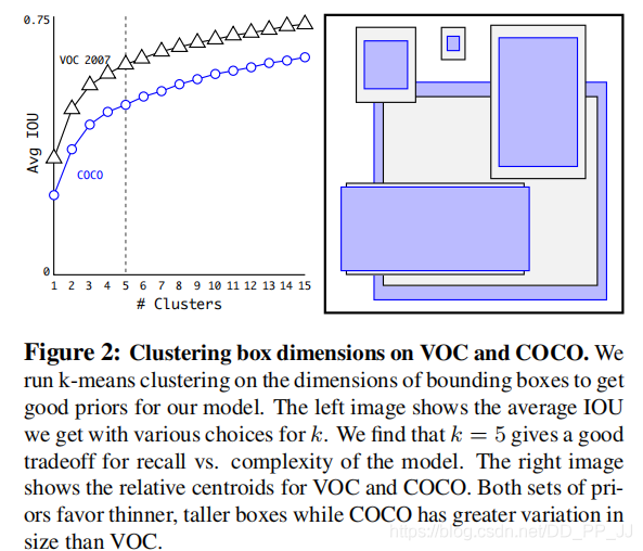
Faster R-CNN中Anchor的大小和比例是由人手工设计的,可能并不贴合数据集,有可能会给模型性能带来负面影响。YOLOv2和YOLOv3则是通过聚类算法得到最适合的k个框。聚类距离是通过IoU来定义,IoU越大,边框距离越近。
Anchor越多,平均IoU会越大,效果越好,但是会带来计算量上的负担,下图是YOLOv2论文中的聚类数量和平均IoU的关系图,在YOLOv2中选择了5个anchor作为精度和速度的平衡。
2. 偏移公式
在Faster RCNN中,中心坐标的偏移公式是:
其中x_a、y_a 代表中心坐标,w_a和h_a代表宽和高,t_x和t_y是模型预测的Anchor相对于Ground Truth的偏移量,通过计算得到的x,y就是最终预测框的中心坐标。
而在YOLOv2和YOLOv3中,对偏移量进行了限制,如果不限制偏移量,那么边框的中心可以在图像任何位置,可能导致训练的不稳定。
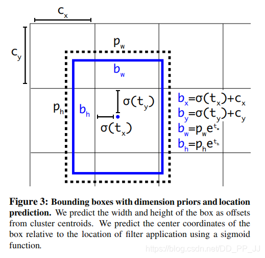
对照上图进行理解:
- c_x和c_y分别代表中心点所处区域的左上角坐标。
- p_w和p_h分别代表Anchor的宽和高。
- \sigma(t_x)和\sigma(t_y)分别代表预测框中心点和左上角的距离,\sigma代表sigmoid函数,将偏移量限制在当前grid中,有利于模型收敛。
-
t_w和t_h代表预测的宽高偏移量,Anchor的宽和高乘上指数化后的宽高,对Anchor的长宽进行调整。
-
\sigma(t_o)是置信度预测值,是当前框有目标的概率乘以bounding box和ground truth的IoU的结果
3. Loss
YOLOv3中有一个参数是ignore_thresh,在ultralytics版版的YOLOv3中对应的是train.py文件中的iou_t参数(默认为0.225)。
正负样本是按照以下规则决定的:
-
如果一个预测框与所有的Ground Truth的最大IoU<ignore_thresh时,那这个预测框就是负样本。
-
如果Ground Truth的中心点落在一个区域中,该区域就负责检测该物体。将与该物体有最大IoU的预测框作为正样本(注意这里没有用到ignore thresh,即使该最大IoU<ignore thresh也不会影响该预测框为正样本)
在YOLOv3中,Loss分为三个部分:
- 一个是xywh部分带来的误差,也就是bbox带来的loss
- 一个是置信度带来的误差,也就是obj带来的loss
- 最后一个是类别带来的误差,也就是class带来的loss
在代码中分别对应lbox, lobj, lcls,yolov3中使用的loss公式如下:
其中:
S: 代表grid size, S^2代表13x13,26x26, 52x52
B: box
1_{i,j}^{obj}: 如果在i,j处的box有目标,其值为1,否则为0
1_{i,j}^{noobj}: 如果在i,j处的box没有目标,其值为1,否则为0
BCE(binary cross entropy)具体计算公式如下:
以上是论文中yolov3对应的darknet。而pytorch版本的yolov3改动比较大,有较大的改动空间,可以通过参数进行调整。
分成三个部分进行具体分析:
1. lbox部分
在ultralytics版版的YOLOv3中,使用的是GIOU,具体讲解见GIOU讲解链接。
简单来说是这样的公式,IoU公式如下:
而GIoU公式如下:
其中A_c代表两个框最小闭包区域面积,也就是同时包含了预测框和真实框的最小框的面积。
yolov3中提供了IoU、GIoU、DIoU和CIoU等计算方式,以GIoU为例:
if GIoU:  # Generalized IoU https://arxiv.org/pdf/1902.09630.pdf
    c_area = cw * ch + 1e-16  # convex area
    return iou - (c_area - union) / c_area  # GIoU
可以看到代码和GIoU公式是一致的,再来看一下lbox计算部分:
giou = bbox_iou(pbox.t(), tbox[i],
                x1y1x2y2=False, GIoU=True)
lbox += (1.0 - giou).sum() if red == 'sum' else (1.0 - giou).mean()
可以看到box的loss是1-giou的值。
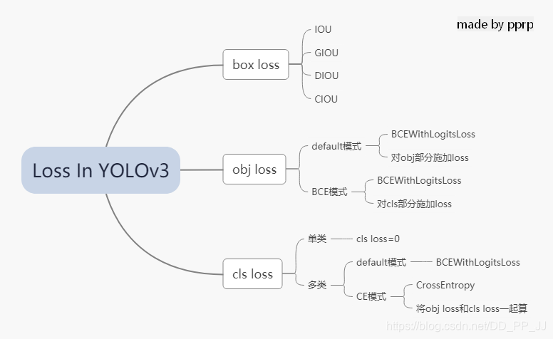
2. lobj部分
lobj代表置信度,即该bounding box中是否含有物体的概率。在yolov3代码中obj loss可以通过arc来指定,有两种模式:
如果采用default模式,使用BCEWithLogitsLoss,将obj loss和cls loss分开计算:
BCEobj = nn.BCEWithLogitsLoss(pos_weight=ft([h['obj_pw']]), reduction=red)
if 'default' in arc:  # separate obj and cls
    lobj += BCEobj(pi[..., 4], tobj)  # obj loss
    # pi[...,4]对应的是该框中含有目标的置信度,和giou计算BCE
    # 相当于将obj loss和cls loss分开计算
如果采用BCE模式,使用的也是BCEWithLogitsLoss, 计算对象是所有的cls loss:
BCE = nn.BCEWithLogitsLoss(reduction=red)
elif 'BCE' in arc:  # unified BCE (80 classes)
    t = torch.zeros_like(pi[..., 5:])  # targets
    if nb:
        t[b, a, gj, gi, tcls[i]] = 1.0 # 对应正样本class置信度设置为1
        lobj += BCE(pi[..., 5:], t)#pi[...,5:]对应的是所有的class
3. lcls部分
如果是单类的情况,cls loss=0
如果是多类的情况,也分两个模式:
如果采用default模式,使用的是BCEWithLogitsLoss计算class loss。
BCEcls = nn.BCEWithLogitsLoss(pos_weight=ft([h['cls_pw']]), reduction=red)
# cls loss 只计算多类之间的loss,单类不进行计算
if 'default' in arc and model.nc > 1:
    t = torch.zeros_like(ps[:, 5:])  # targets
    t[range(nb), tcls[i]] = 1.0 # 设置对应class为1
    lcls += BCEcls(ps[:, 5:], t)  # 使用BCE计算分类loss
如果采用CE模式,使用的是CrossEntropy同时计算obj loss和cls loss。
CE = nn.CrossEntropyLoss(reduction=red)
elif 'CE' in arc:  # unified CE (1 background + 80 classes)
    t = torch.zeros_like(pi[..., 0], dtype=torch.long)  # targets
    if nb:
    t[b, a, gj, gi] = tcls[i] + 1 # 由于cls是从零开始计数的,所以+1
    lcls += CE(pi[..., 4:].view(-1, model.nc + 1), t.view(-1))
    # 这里将obj loss和cls loss一起计算,使用CrossEntropy Loss
以上三部分总结下来就是下图:
4. 代码
ultralytics版版的yolov3的loss已经和论文中提出的部分大相径庭了,代码中很多地方地方是来自作者的经验。另外,这里读的代码是2020年2月份左右作者发布的版本,关注这个库的人会知道,作者更新速度非常快,在笔者写这篇文章的时候,loss也出现了大幅改动,添加了label smoothing等新的机制,去掉了通过arc来调整loss的机制,简化了loss部分。
这部分的代码添加了大量注释,很多是笔者通过debug得到的结果,理解的时候需要讲一下debug的配置:
- 单类数据集class=1
- batch size=2
- 模型是yolov3.cfg
计算loss这部分代码可以大概上分为两部分,一部分是正负样本选取,一部分是loss计算。
1. 正负样本选取部分
这部分主要工作是在每个yolo层将预设的anchor和ground truth进行匹配,得到正样本,回顾一下上文中在YOLOv3中正负样本选取规则:
-
如果一个预测框与所有的Ground Truth的最大IoU<ignore_thresh时,那这个预测框就是负样本。
-
如果Ground Truth的中心点落在一个区域中,该区域就负责检测该物体。将与该物体有最大IoU的预测框作为正样本(注意这里没有用到ignore thresh,即使该最大IoU<ignore thresh也不会影响该预测框为正样本)
def build_targets(model, targets):
    # targets = [image, class, x, y, w, h]
    # 这里的image是一个数字,代表是当前batch的第几个图片
    # x,y,w,h都进行了归一化,除以了宽或者高

    nt = len(targets)

    tcls, tbox, indices, av = [], [], [], []

    multi_gpu = type(model) in (nn.parallel.DataParallel,
                                nn.parallel.DistributedDataParallel)

    reject, use_all_anchors = True, True
    for i in model.yolo_layers:
        # yolov3.cfg中有三个yolo层,这部分用于获取对应yolo层的grid尺寸和anchor大小
        # ng 代表num of grid (13,13) anchor_vec [[x,y],[x,y]]
        # 注意这里的anchor_vec: 假如现在是yolo第一个层(downsample rate=32)
        # 这一层对应anchor为:[116, 90], [156, 198], [373, 326]
        # anchor_vec实际值为以上除以32的结果:[3.6,2.8],[4.875,6.18],[11.6,10.1]
        # 原图 416x416 对应的anchor为 [116, 90]
        # 下采样32倍后 13x13 对应的anchor为 [3.6,2.8]
        if multi_gpu:
            ng = model.module.module_list[i].ng
            anchor_vec = model.module.module_list[i].anchor_vec
        else:
            ng = model.module_list[i].ng,
            anchor_vec = model.module_list[i].anchor_vec

        # iou of targets-anchors
        # targets中保存的是ground truth
        t, a = targets, []

        gwh = t[:, 4:6] * ng[0]

        if nt:  # 如果存在目标
            # anchor_vec: shape = [3, 2] 代表3个anchor
            # gwh: shape = [2, 2] 代表 2个ground truth
            # iou: shape = [3, 2] 代表 3个anchor与对应的两个ground truth的iou
            iou = wh_iou(anchor_vec, gwh)  # 计算先验框和GT的iou

            if use_all_anchors:
                na = len(anchor_vec)  # number of anchors
                a = torch.arange(na).view(
                    (-1, 1)).repeat([1, nt]).view(-1)  # 构造 3x2 -> view到6
                # a = [0,0,1,1,2,2]
                t = targets.repeat([na, 1])
                # targets: [image, cls, x, y, w, h]
                # 复制3个: shape[2,6] to shape[6,6]
                gwh = gwh.repeat([na, 1])
                # gwh shape:[6,2]
            else:  # use best anchor only
                iou, a = iou.max(0)  # best iou and anchor
                # 取iou最大值是darknet的默认做法,返回的a是下角标

            # reject anchors below iou_thres (OPTIONAL, increases P, lowers R)
            if reject:
                # 在这里将所有阈值小于ignore thresh的去掉
                j = iou.view(-1) > model.hyp['iou_t']
                # iou threshold hyperparameter
                t, a, gwh = t[j], a[j], gwh[j]

        # Indices
        b, c = t[:, :2].long().t()  # target image, class
        # 取的是targets[image, class, x,y,w,h]中 [image, class]

        gxy = t[:, 2:4] * ng[0]  # grid x, y

        gi, gj = gxy.long().t()  # grid x, y indices
        # 注意这里通过long将其转化为整形,代表格子的左上角

        indices.append((b, a, gj, gi))
        # indice结构体保存内容为:
        '''
        b: 一个batch中的角标
        a: 代表所选中的正样本的anchor的下角标
        gj, gi: 代表所选中的grid的左上角坐标
        '''
        # Box
        gxy -= gxy.floor()  # xy
        # 现在gxy保存的是偏移量,是需要YOLO进行拟合的对象
        tbox.append(torch.cat((gxy, gwh), 1))  # xywh (grids)
        # 保存对应偏移量和宽高(对应13x13大小的)
        av.append(anchor_vec[a])  # anchor vec
        # av 是anchor vec的缩写,保存的是匹配上的anchor的列表

        # Class
        tcls.append(c)
        # tcls用于保存匹配上的类别列表
        if c.shape[0]:  # if any targets
            assert c.max() < model.nc, 'Model accepts %g classes labeled from 0-%g, however you labelled a class %g. ' \
                                       'See https://github.com/ultralytics/yolov3/wiki/Train-Custom-Data' % (
                                           model.nc, model.nc - 1, c.max())
    return tcls, tbox, indices, av
梳理一下在每个YOLO层的匹配流程:
- 将ground truth和anchor进行匹配,得到iou
- 然后有两个方法匹配:
- 使用yolov3原版的匹配机制,仅仅选择iou最大的作为正样本
- 使用ultralytics版版yolov3的默认匹配机制,use_all_anchors=True的时候,选择所有的匹配对
- 对以上匹配的部分在进行筛选,对应原版yolo中ignore_thresh部分,将以上匹配到的部分中iou<ignore_thresh的部分筛选掉。
- 最后将匹配得到的内容返回到compute_loss函数中。
2. loss计算部分
这部分就是yolov3中核心loss计算,这部分对照上文的讲解进行理解。
def compute_loss(p, targets, model):
    # p: (bs, anchors, grid, grid, classes + xywh)
    # predictions, targets, model
    ft = torch.cuda.FloatTensor if p[0].is_cuda else torch.Tensor
    lcls, lbox, lobj = ft([0]), ft([0]), ft([0])
    tcls, tbox, indices, anchor_vec = build_targets(model, targets)
    '''
    以yolov3为例,有三个yolo层
    tcls: 一个list保存三个tensor,每个tensor中有6(2个gtx3个anchor)个代表类别的数字
    tbox: 一个list保存三个tensor,每个tensor形状[6,4],6(2个gtx3个anchor)个bbox
    indices: 一个list保存三个tuple,每个tuple中保存4个tensor:
            分别代表        b: 一个batch中的角标
                            a: 代表所选中的正样本的anchor的下角标
                            gj, gi: 代表所选中的grid的左上角坐标
    anchor_vec: 一个list保存三个tensor,每个tensor形状[6,2],
                6(2个gtx3个anchor)个anchor,注意大小是相对于13x13feature map的anchor大小
    '''

    h = model.hyp  # hyperparameters
    arc = model.arc  # # (default, uCE, uBCE) detection architectures
    # 具体使用的损失函数是通过arc参数决定的
    red = 'sum'  # Loss reduction (sum or mean)

    # Define criteria
    BCEcls = nn.BCEWithLogitsLoss(pos_weight=ft([h['cls_pw']]), reduction=red)
    BCEobj = nn.BCEWithLogitsLoss(pos_weight=ft([h['obj_pw']]), reduction=red)
    #BCEWithLogitsLoss = sigmoid + BCELoss
    BCE = nn.BCEWithLogitsLoss(reduction=red)
    CE = nn.CrossEntropyLoss(reduction=red)  # weight=model.class_weights

    # class label smoothing https://arxiv.org/pdf/1902.04103.pdf eqn 3
    # cp, cn = smooth_BCE(eps=0.0)
    # 这是最新的版本中提供了label smoothing的功能,只能用在多类问题

    if 'F' in arc:  # add focal loss
        g = h['fl_gamma']
        BCEcls, BCEobj, BCE, CE = FocalLoss(BCEcls, g), FocalLoss(
            BCEobj, g), FocalLoss(BCE, g), FocalLoss(CE, g)
        # focal loss可以用在cls loss或者obj loss

    # Compute losses
    np, ng = 0, 0  # number grid points, targets
    # np这个命名真的迷,建议改一下和numpy缩写重复
    for i, pi in enumerate(p):  # layer index, layer predictions
        # 在yolov3中,p有三个yolo layer的输出pi
        # 形状为:(bs, anchors, grid, grid, classes + xywh)
        b, a, gj, gi = indices[i]  # image, anchor, gridy, gridx
        tobj = torch.zeros_like(pi[..., 0])
        # tobj = target obj, 形状为(bs, anchors, grid, grid)
        np += tobj.numel() # 返回tobj中元素个数

        # Compute losses
        nb = len(b)
        if nb:
            ng += nb # number of targets 用于最后算平均loss
            # (bs, anchors, grid, grid, classes + xywh)
            ps = pi[b, a, gj, gi] # 即找到了对应目标的classes+xywh,形状为[6(2x3),6]

            # GIoU
            pxy = torch.sigmoid(
                ps[:, 0:2] # 将x,y进行sigmoid
            )  # pxy = pxy * s - (s - 1) / 2,  s = 1.5  (scale_xy)
            pwh = torch.exp(ps[:, 2:4]).clamp(max=1E3) * anchor_vec[i]
            # 防止溢出进行clamp操作,乘以13x13feature map对应的anchor
            # 这部分和上文中偏移公式是一致的
            pbox = torch.cat((pxy, pwh), 1)  # predicted box
            # pbox: predicted bbox shape:[6, 4]
            giou = bbox_iou(pbox.t(), tbox[i], x1y1x2y2=False,
                            GIoU=True)  # giou computation
            # 计算giou loss, 形状为6
            lbox += (1.0 - giou).sum() if red == 'sum' else (1.0 - giou).mean()
            # bbox loss直接由giou决定
            tobj[b, a, gj, gi] = giou.detach().type(tobj.dtype)
            # target obj 用giou取代1,代表该点对应置信度

            # cls loss 只计算多类之间的loss,单类不进行计算
            if 'default' in arc and model.nc > 1:
                t = torch.zeros_like(ps[:, 5:])  # targets
                t[range(nb), tcls[i]] = 1.0 # 设置对应class为1
                lcls += BCEcls(ps[:, 5:], t)  # 使用BCE计算分类loss

        if 'default' in arc:  # separate obj and cls
            lobj += BCEobj(pi[..., 4], tobj)  # obj loss
            # pi[...,4]对应的是该框中含有目标的置信度,和giou计算BCE
            # 相当于将obj loss和cls loss分开计算

        elif 'BCE' in arc:  # unified BCE (80 classes)
            t = torch.zeros_like(pi[..., 5:])  # targets
            if nb:
                t[b, a, gj, gi, tcls[i]] = 1.0 # 对应正样本class置信度设置为1
            lobj += BCE(pi[..., 5:], t)
            #pi[...,5:]对应的是所有的class

        elif 'CE' in arc:  # unified CE (1 background + 80 classes)
            t = torch.zeros_like(pi[..., 0], dtype=torch.long)  # targets
            if nb:
                t[b, a, gj, gi] = tcls[i] + 1 # 由于cls是从零开始计数的,所以+1
            lcls += CE(pi[..., 4:].view(-1, model.nc + 1), t.view(-1))
            # 这里将obj loss和cls loss一起计算,使用CrossEntropy Loss
    # 使用对应的权重来平衡,这个参数是作者通过参数搜索(random search)的方法搜索得到的
    lbox *= h['giou']
    lobj *= h['obj']
    lcls *= h['cls']

    if red == 'sum':
        bs = tobj.shape[0]  # batch size
        lobj *= 3 / (6300 * bs) * 2
        # 6300 = (10 ** 2 + 20 ** 2 + 40 ** 2) * 3
        # 输入为320x320的图片,则存在6300个anchor
        # 3代表3个yolo层, 2是一个超参数,通过实验获取
        # 如果不想计算的话,可以修改red='mean'
        if ng:
            lcls *= 3 / ng / model.nc
            lbox *= 3 / ng
    loss = lbox + lobj + lcls
    return loss, torch.cat((lbox, lobj, lcls, loss)).detach()
需要注意的是,三个部分的loss的平衡权重不是按照yolov3原文的设置来做的,是通过超参数进化来搜索得到的,具体请看:【从零开始学习YOLOv3】4. YOLOv3中的参数进化
5. 补充
补充一下BCEWithLogitsLoss的用法,在这之前先看一下BCELoss:
torch.nn.BCELoss的功能是二分类任务是的交叉熵计算函数,可以认为是CrossEntropy的特例。其分类限定为二分类,y的值必须为{0,1},input应该是概率分布的形式。在使用BCELoss前一般会先加一个sigmoid激活层,常用在自编码器中。
计算公式:
w_n是每个类别的loss权重,用于类别不均衡问题。
torch.nn.BCEWithLogitsLoss的相当于Sigmoid+BCELoss, 即input会经过Sigmoid激活函数,将input变为概率分布的形式。
计算公式:
本文总阅读量次